Assessment of Storm Surge and Flood Inundation in Chittagong City of Bangladesh Based on ADCIRC and GIS

LIU Yuxin, LI Songtao, and WANG Zhifeng

Assessment of Storm Surge and Flood Inundation in Chittagong City of Bangladesh Based on ADCIRC and GIS

LIU Yuxin1), LI Songtao2), *, and WANG Zhifeng2)

1) National Ocean Technology Center, Tianjin 300110, China 2) Shandong Provincial Key Laboratory of Ocean Engineering & College of Engineering, Ocean University of China,Qingdao 266100, China

Coastal flooding caused by tropical cyclones has long been a major threat to life, property, and infrastructure in coastal zones. This study assessed the risk of flooding in Chittagong, southeastern Bangladesh, under extreme sea level scenarios caused by high astronomical tides and storm surges. The Jelesnianski typhoon model and the ADvanced CIRCulation hydrodynamic model were used to simulate 91 typhoons that occurred in the Bay of Bengal between 1981 and 2017, and observational data were used for model validation. The inundation model was based on a digital elevation model and a seed spread algorithm, and a geographical information system was used to visualize the flood risk. Under four scenarios, the changes in flood levels caused by sea level rise had no significant influence on the extent of flooding in Chittagong. At flood levels of 8.82m (50-year storm surge without sea level rise) and 8.89m (50-year storm surge with sea level rise), the maximum estimated area of inundation was 11.35km2. The western coastal and southeastern river coastal plain areas of Chittagong have the highest risk of inundation due to their low-lying terrain. At flood levels of 9.83m (100-year storm surge without sea level rise) and 9.97m (100-year storm surge with sea level rise), the maximum simulated flood extent was 36.44km2. Simulated floodwaters propagated in a south–north direction, and most of the northern areas of the city are at risk of inundation under these scenarios.

typhoon; storm surge; extreme sea level; inundation

1 Introduction

Coastal flooding can have significant damaging impacts on any coastal zone, which can occur due to sea level rise and is frequently associated with energetic events, including tropical cyclones (Nicholls, 1999). The consequences of coastal flooding can lead to the loss of life and damage to property and critical infrastructure. Meteorological events such as cyclones can result in severe storm surges that cause abnormal rises in water levels that are higher than the regular astronomical tide levels and are capable of flooding large coastal areas (Bhaskaran, 2014). The total water level that affects flood hazard receptors (, people) and defense fragility (, the pathway to the receptors) is a combination of tide, surge, and wave effects. The combination of these physical processes must be included; however, it is further complicated by theinteraction of these physical processes (Lewis, 2019). In recent years, sea level rise due to climate change has become an additional pressure that increases the risk of coastal flooding (Nicholls, 2002). Over the past two centuries, approximately two million people worldwide have died and millions have been injured as a result of tropical storms (cyclones, hurricanes, and typhoons) (Ubydul, 2012).Storm surges are an important factor that leads to coastal flooding. Whether a storm surge becomes a disaster depends largely on whether a storm surge peak coincides with high astronomical tides.Other factors contribute to the risk level, including the geographical area where these events occur, the shape of the coastline, the topography of the shoreline and seabed, and, in particular, the social and economic status of the inundated areas. To further reduce storm surge fatalities, improved coastal flood riskestimatesshouldbeprioritized,requiringaccuratequan- tification of storm surge characteristics. With the rapid advancement in numerical models and computing power, different high-resolution mesoscale models are being increasingly used for the prediction of tropical cyclones. Over the years, several researchers (Dietrich, 2011; Zheng, 2013; Bhaskaran, 2014) have developed and adopted various numerical models (, IITD model; SLOSH; ADCIRC; FVCOM) to predict and study the behavior of a storm and estimate the associated surge (particularly along nearshore areas).

Of all the countries on the fringes of the Bay of Bengal, Bangladesh has been most affected by storm surges. Approximately 300000 lives were lost in the severe cyclones that hit the country in November 1970, while approximately 10000 lives were lost as a result of the Andhra cyclone in November 1977. Aside from causing a significant amount of property damage in the region, the Chittagong cyclone of April 1991 claimed approximately 140000 lives, and more than 15000 people were killed during the Odisha super cyclone in October 1999 (Dube, 2009). Most of the damage and deaths caused by these cyclones resulted from storm surge-driven flooding and its associated inland inundation. The development of effective preparedness measures to cope with storm surges is a key factor in minimizing their impact on society.

The extent of flooding resulting from a storm surge depends on the characteristics of the storm and the shape andhydrodynamic behavior of the affected coastal areas.Chittagong is Bangladesh’s largest port city and the second most populous. It has an important economic and political status, but it is often affected by tropical cyclones.To reduce, or ideally avoid, the adverse effects of flooding, the driving factors of floods need to be determined, and predictive flood extent mapping must be undertaken. Detailed reviews of storm surge studies for the Bay of Bengal were conducted by Ali (1979), Rao (1982), Roy (1984), Murty(1986), Das (1994), Dube(1997), Chittibabu (1999), and Gonnert(2001).

This study aimed to assess the risk of flooding in Chit- tagong on the basis of data from 91 typhoons that occurredin the Bay of Bengal between 1981 and 2017. This assess- ment was performed by developing wind fields and pres- sure fields based on the Jelesnianski model and by simu- lating astronomical tides and storm surges using the AD- vanced CIRCulation (ADCIRC) hydrodynamic model.On the basis of a seed spread algorithm, an inundation model was then used to determine the flood inundation extent for Chittagong, which was visualized using a geographical in- formation system (GIS).

2 Data and Methods

2.1 Digital Elevation Model Data

A digital elevation model (DEM) is a solid ground mod- el that expresses the ground elevation in the form of agroup of ordered numerical arrays, thereby realizing thedigital simulation of the ground terrain through limited ter-rain elevation data. The datasets used to construct the DEM were obtained from the Chinese Academy of Sciences Computer Network Information Center(http://www.gscloud.cn/). These data were processed using Advanced Spaceborne Thermal Emission and Reflection Radiometer Global DEM (ASTER GDEM) (ver. 1) and digital elevation data with a global spatial resolution of 30m.ASTER GDEM was jointly launched by NASA and METI in June 2009. The terrain data are based on detailed observations of NASA’s new Earth observation satellite Terra. The data covered up to 99% of the land area between 83?S and 83?N. ASTER GDEM data were fragmented into 1? grid cellscontaining 22600 fragment data files, which are distributed in GeoTIFF format using the WGS1984 projection. Each pixel was 1 rad (1 radian,30m), and the elevation was based on the EGM96 global quasi-geoid model. TheEGM96 model is one of the most frequently used Earth gravity field models. It is a series of global high-order and ultrahigh-order Earth gravity field models obtained by using ground gravity data, satellite altimetry data, CHAMP, and GRACE satellite tracking data.

Prior to the analysis, the DEM was checked for errors, including the existence of artificial surface depressions and positive terrain elements that would have affected the direction of the simulated water flow. These errors were then corrected. In view of this situation, the method of filling depressions is generally adopted to obtain DEM without depressions.DEM is considered a relatively smooth terrain surface simulation, but due to interpolation and the existence of some special terrain (such as karst landform), some depressed areas are often found on the DEM surface. During hydrologic analysis in these areas, unreasonable or even wrong water flow direction is easily obtained due to the presence of low-elevation grids. Therefore, before the calculation of hydrologic analysis, depression-free DEM should be obtained by filling the depressions of the original DEM data first.

2.2 Jelesnianski Typhoon Model

Numerical-based typhoon models are an indispensable part of typhoon research. Their accuracy directly determines the reliability of typhoon storm surge simulations.Wind stress and horizontal gradients of surface atmospheric pressure are the main drivers of storm surges (Pan- dey and Rao, 2018).In recent years, many numerical models have been developed using the Jelesnianski typhoon model to calculate wind field distributions (Jain, 2010; Rao, 2010, 2013, 2020; Murty, 2014; Wang, 2019).

The wind field element of the Jelesnianski typhoon model (Jelesnianski, 1966) can be decomposed into two vector fields. Solving the wind field is equivalent to solving the wind field of circular typhoons and moving typhoons, and the solution formula is as follows:

whereis the calculating point wind speed;Vis the circular wind speed; andVis the moving wind speed.

The model assumes that the wind speed of a circular typhoon wind field is distributed according to a certain law and that the wind field is circularly symmetrical. When the center position, maximum near-center wind speed, and maximum wind speed radius of a typhoon are known at different points in time, the circular typhoon wind field can be calculated as follows:

where

whereis the maximum wind radius;Vis the maximum typhoon wind speed;is the distance from the calculating point to the typhoon center;is the zonal distance from the calculating point to the typhoon center;is the meridional distance from the calculating point to the typhoon center;is the unit vector in thedirection;is the unit vector in the-direction; andis the fluid inlet angle, where=20?.

Typhoons move along certain paths. Given the known velocity and maximum wind speed radius of a typhoon, the wind speed in the moving typhoon wind field can be calculated as follows:

whereVis the zonal moving speed of the typhoon center, andVis the meridional moving speed of the typhoon center.

Typhoon pressure field models based on the study of typhoon sea surface pressures are an important part of empirical typhoon models. The calculation formula of the Je- lesnianski pressure field model as used here is as follows:

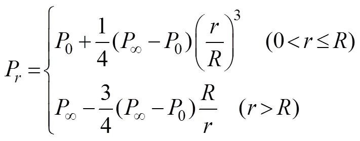
where∞is the peripheral pressure (∞=101kPa), and0is the typhoon central pressure.

A detailed description and validation of the Jelesnianski model are given in Wang(2020).

2.3 ADCIRC Model Introduction

Astronomical tides and storm surges were simulated based on the ADCIRC hydrodynamic model, which has been used to compute tides along the east and west coasts of India by prescribing tidal elevations from the Le Provost tidal constituent database along the open boundary on a real-time basis (Le Provost, 1995). The ADCIRC model was recently successfully applied to simulate storm surges (Hatzikyriakou andLin, 2017; Choi, 2018; Gowri Shankar, 2018).

The ADCIRC model is a finite element model that was developed to simulate hydrodynamic circulations along shelves and coasts (Luettich, 1992; Westerink, 1994), and it can be run as a two-dimensional depth-integrated (2DDI) model or as a three-dimensional model. ADCIRC solves shallow-water equations by using the gen- eralized wave continuity equation (Eq. (6)) and vertically integrated momentum equations (Eqs. (7) and (8)) to solvewater levels and currents, respectively.The ADCIRC model employs the continuous Galerkin finite element method to discretize onto unstructured meshes as follows:

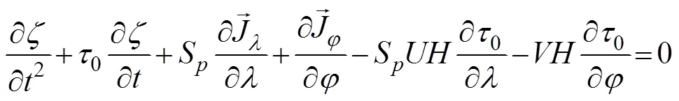
where

Currentsandare obtained from vertically integrated momentum equations as follows:

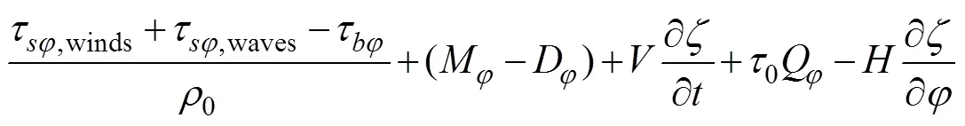
where=+is the total water depth (m);is the deviation of the water surface from the mean (m);is the bathy- metric depth (m);S=cos0/cosφis the spherical coordinate conversion factor (unitless);andare the depth-integrated currents in the- and-directions, respectively;Q=andQ=are the fluxes per unit width (m2s?1);is the Coriolis parameter;is the gravitational acceleration (ms?2);Pis the atmospheric pressure at the surface (Nm?2);0is the reference density of water (kgm?3);is the Newtonian equilibrium tidal potential;is the effective earth elasticity factor;τ,windsandτ,wavesare surface stresses due to winds and waves, respectively (Nm?2);τis the bottom stress (Nm?2);is the lateral stress gradient (Nm?2m?1);is a momentum dispersion term (Nm?2m?1); and0is a numerical parameter that optimizes the phase propagation properties (unitless) (Dietrich, 2012).

2.4 ADCIRC Model Setup and Validation

The ADCIRC model was used to simulate 91 typhoon events by using the data outlined in Section 2.1. The selected simulation area was the coastal area of the Bay of Bengal, covering 82?–95?E and 10?–23?N.The bathymetric data required for the numerical simulation of storm surges (Fig.1) were obtained from the ETOPO1 global topographic database ETOPO1 is a global topographic re- lief model with a resolution of 1? and contains data on land topography and marine water depth.

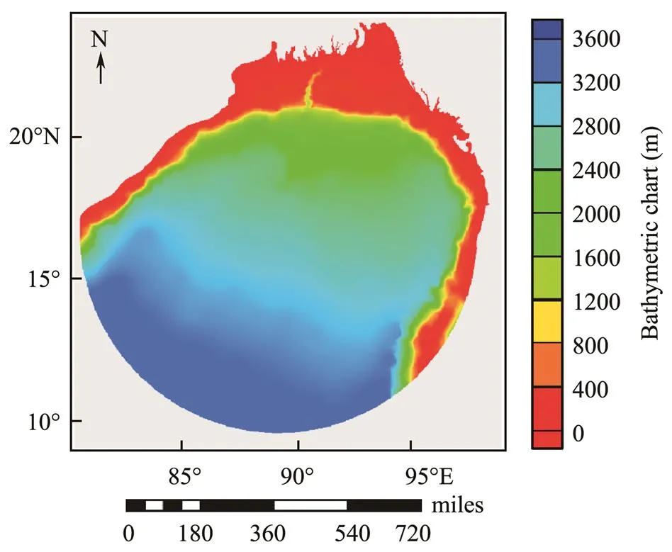
Fig.1 Bathymetric chart for the ADCIRC model simulation region.

A triangular mesh was used in the ADCIRC simulations(Fig.2).Within the simulation area, different resolutions can be selected for different locations according to user needs.The step size of the mesh gradually decreases from offshoreto nearshore, thereby reducing the number of ADCIRC model meshes and the simulation time and improving the simulation accuracy. According tothe mesh division principle of this approach, the offshore mesh has a low resolution, and the nearshore mesh has a high resolution. The triangular mesh has a resolution of about 10km in the open ocean boundary and refines to about 50–100m along the coastal regions.

A minimum depth of 0.05m is prescribed with a horizontal eddy viscosity coefficient of 2m2s?1to delineate the wet and dry elements. The bottom friction coefficient considered for the simulations is 0.0025, obtained by using a hybrid scheme with a model time step of 20s. Wind fields and pressure fields simulated by the Jelesnianski typhoon model were used as the input file.

With the influence of astronomical tides during typhoon landings taken into consideration, eight major harmonic constituents (Q1, O1, P1, K1, N2, M2, S2, and K2) were given on the open boundary.Meteorological forcing data, namely, atmospheric pressure and wind stress information, were derived from the wind fields and pressure fields that were simulated using the Jelesnianski model. This model inputs the location of the typhoon center, the maximum wind speed in the typhoon center, and other baseline data from the Joint Typhoon Warning Center (JTWC).

To validate the results of the ADCIRC model, we selected five water level stations (https://uhslc.soest.hawaii.edu) as validation points: 1) Hiron point; 2) Chittagong; 3) Cox’s Bazaar; 4) Charchanga; and 5) Khepupara (Fig.3).With the influence of extreme weather and limited measured data, typhoons 8304, 8501, 8804, 9504, and 1601 (Fig.3) were used as example events to validate the astronomical tide and storm surge estimations.

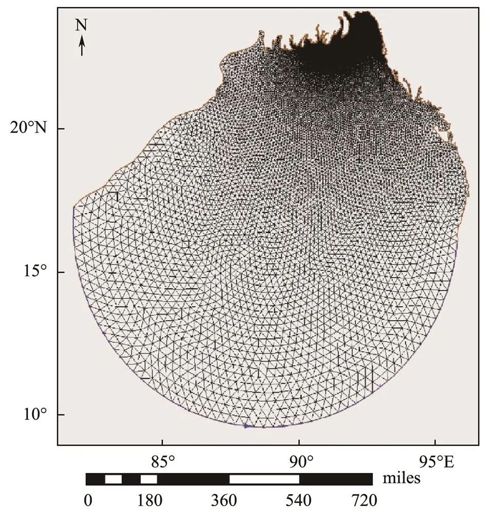
Fig.2 Triangular meshes of the ADCIRC model calculation region.

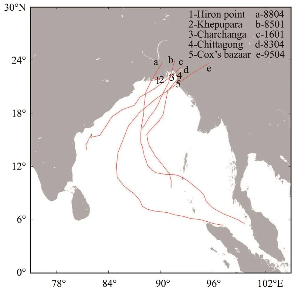
Fig.3 Location of water level stations and typhoon paths.

First, the astronomical tides during the five typhoon months were validated. Table 1 shows the comparison results for the amplitudes and phases of the astronomical tideof each observation station (https://uhslc.soest.hawaii.edu), and Fig.4 shows the validation results for the astronomi- cal tide level at each observation station.The simulation results were in good agreement with the observed data.The same five typhoons were used to validate the accuracy of the ADCIRC model in simulating storm surges, as shown in Fig.5.Again, the simulation results were in good agreement with the observational data, indicating that the ADC- IRC model can effectively simulate storm surges in the northern part of the Bay of Bengal.

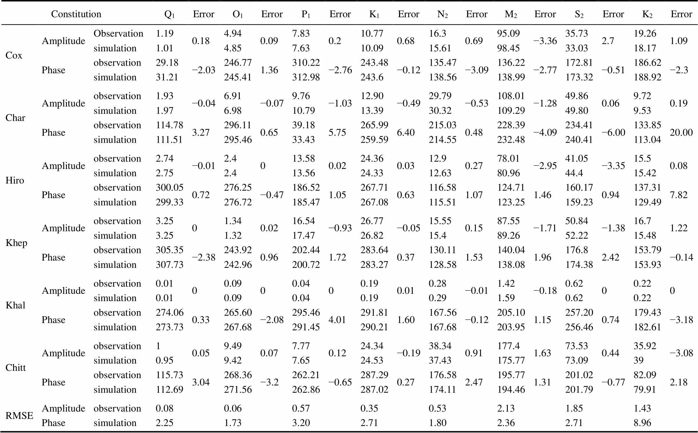
Table 1 Validation of the amplitudes and phases of eight harmonic model constituents

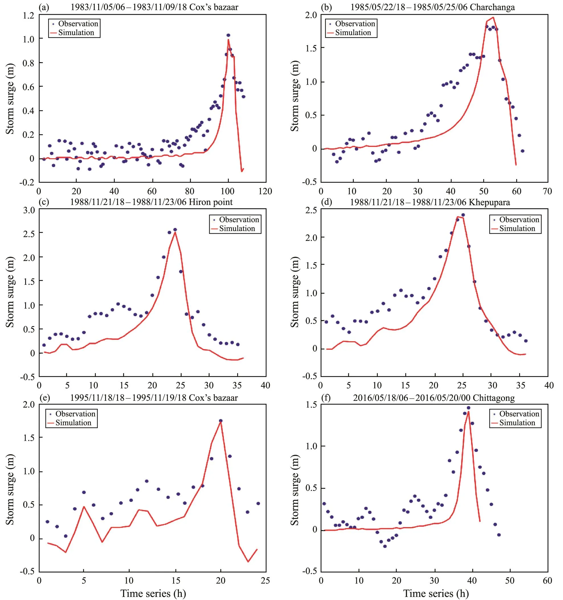
Fig.5 Validation of storm surges during five typhoon events.

3 Results and Discussion

3.1 Analysis of Typhoon Data and Characteristics

Tropical cyclone information was obtained every 6h from the JTWC for the period 1981–2017.A total of 91 tropical cyclones affected the Bay of Bengal during this period (Fig.6), with a maximum of seven in 1992 andan annual average of 2.5. Fig.7 shows that the annual number of tropical cyclones in this region (Fig.7a) has a linearly downward trend with a rate of 0.0284.On the basis of the three-year moving average, the annual frequency of typhoons in this region shows a generally downward fluc- tuating trend.An analysis of the variation in typhoon intensity over the last 37 years (Fig.7b) shows that the intensity of typhoons in the Bay of Bengal exhibited an initial upward trend, then downward, and then upward again. The overall mean maximum wind speed during this period shows a slight upward trend with a rate of 0.0185.

Fig.8 shows the intermonthly distribution of typhoons in the Bay of Bengal, which displays a bimodal distribution with peaks in May and October/November. The winter monsoon is active between January and April, and the summer monsoon is active between June and September, when tropical cyclones occur less frequently. No tropical cyclones occurred in March and August.

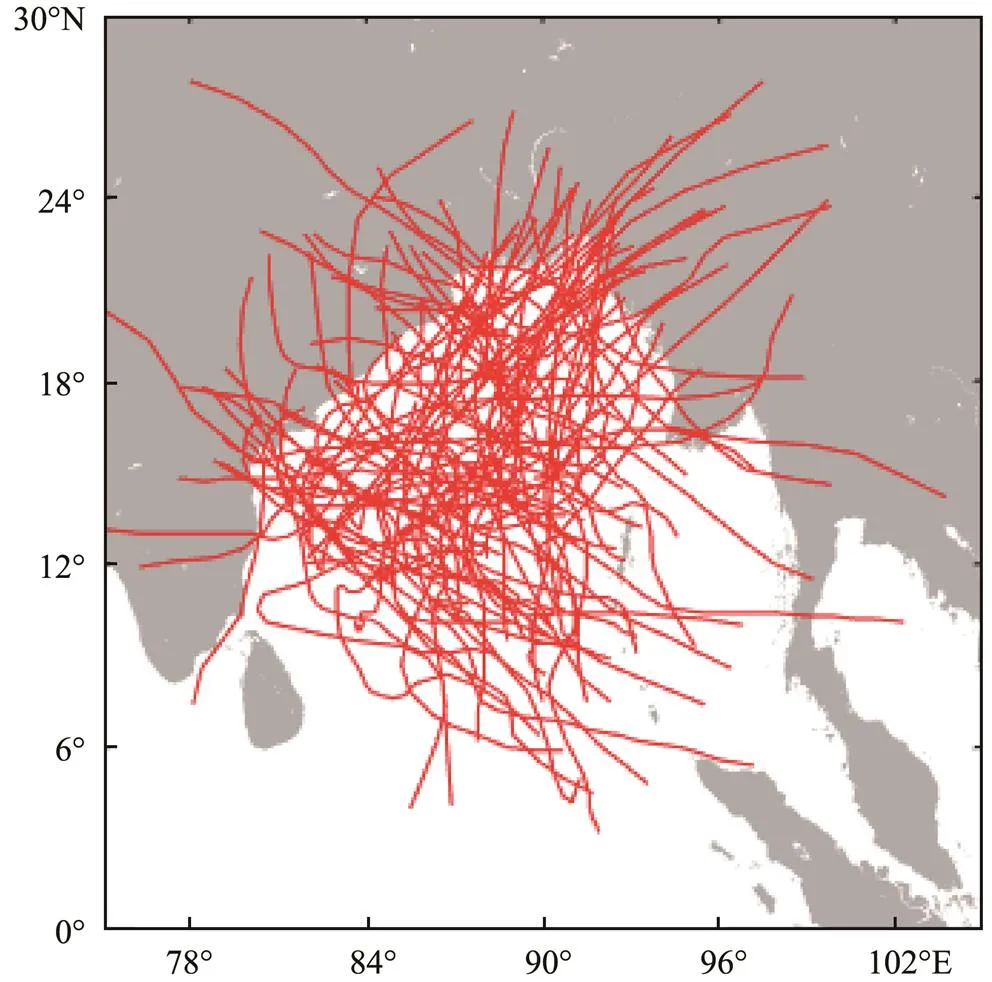
Fig.6 Typhoon tracks in the Bay of Bengal between 1981 and 2017.

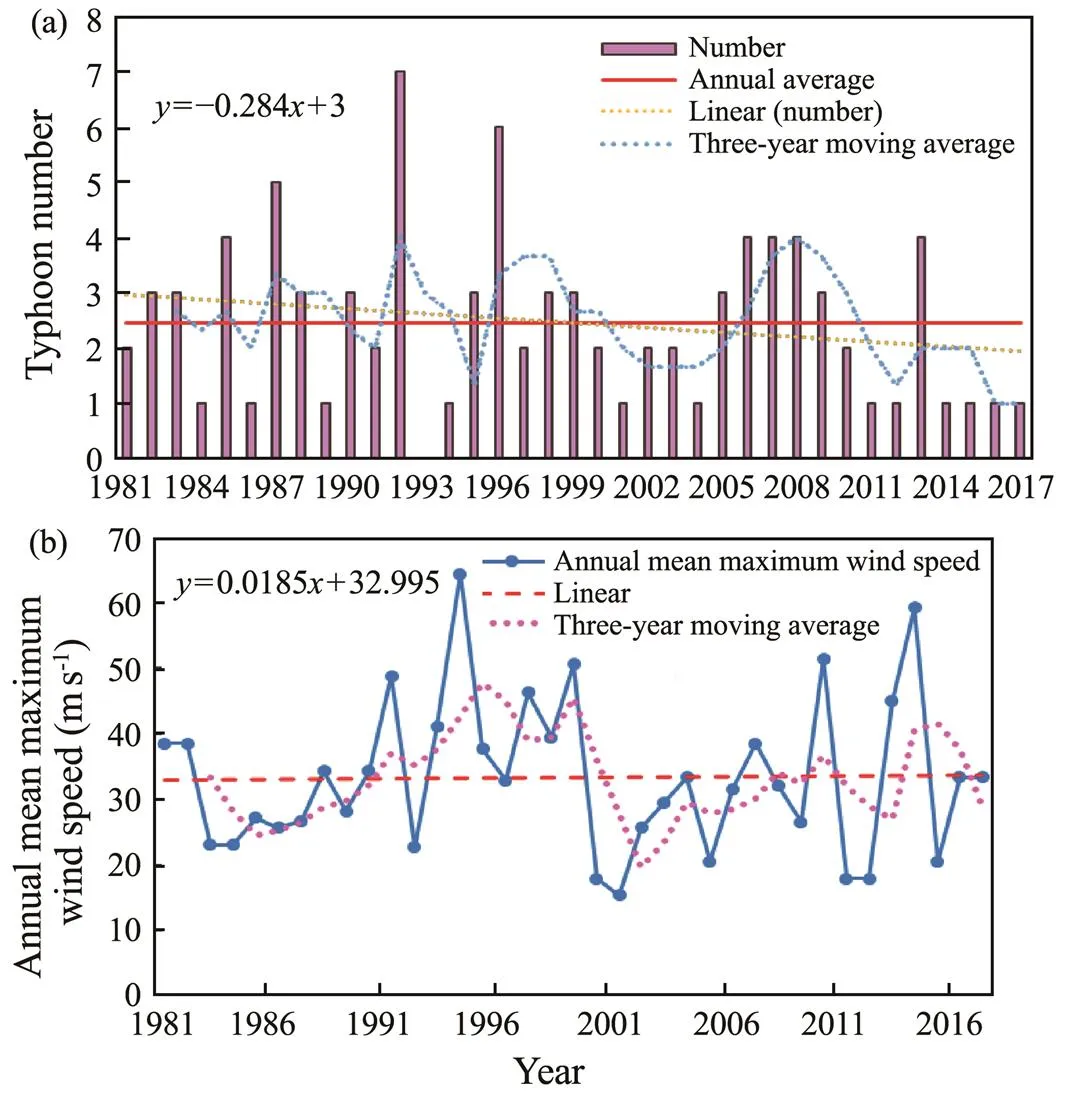
Fig.7 Variation in the number (a) and intensity (b) of tropical cyclones in the Bay of Bengal between 1981 and 2017.

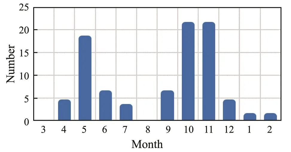
Fig.8 Intermonthly variation of the occurrence of tropical storms in the Bay of Bengal between 1981 and 2017.

3.2 Storm Surge

For the traditional annual extreme method, only one max- imum value is selected as the sample series for calculation. Therefore, the calculation error is large in the case of short statistic years, and selecting a better theoretical frequency curve fitting with the empirical point is difficult. In recent years, the peak-over-threshold (POT) approach has been widely used, in which all the data that reach or exceed a certain fixed large value (threshold) can be selected as the sample for probability analysis. The POT approach was used to sample the storm surge of the 91 typhoon eventsduring the study period. The POT approach was recently applied to determine return water levels in northern Germany (Arns, 2015), and it was used specifically for storm surges by Tebaldi(2012) along the coastlines of the USA; by Hallegatte(2011) in Copenhagen, Denmark; and by Bernardara(2011) along the Atlantic French coast. The POT distribution of generalized extreme values is the generalized Pareto distribution (GPD), which is expressed as follows:

from which the following relationship is obtained:

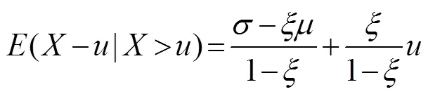
whereis the threshold;is the shape parameter;is the scale parameter; and(–|>)is the expected value of the threshold excess

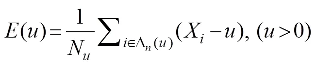
where()is the sample mean exceedance function; Nis the number of the thresholdexceeded in the sample; and?()is the subscript set of observed values exceeding.

As the expected value is approximate to the mean value, the scatter distribution graph (, the mean excess life diagram) of the threshold–the mean value (, the mean excess value) of the observed value (–|>) can be derived according to Eq. (12). When the shape parameteris stable, the graph is approximately a straight line,, the thresholdis taken as the horizontal axis, and the meanvalue of the supra-threshold is taken as the vertical axis. The slope and intercept of the line are(1?), (?)/(1?). Therefore, the range of the abscissa corresponding to the straight-line segment in the graph can be used as the optional range of the threshold (Stuart andJonathan, 1991).On the basis of this approach, a diagnostic test can further determine the threshold and test its rationality.

On the basis of available observations, the hourly measured water level data from Chittagong Station (https://uhslc.soest.hawaii.edu) for the period of May to October 2007–2017 were used for the POT approach in Chittagong.Withthe influence of different seasons on the measured data and the intermonthly variation in typhoon occurrence in the Bay of Bengal taken into consideration, three main factors that influence the water levels in Chittagong were identified: monthly mean sea level, astronomical tides, and storm surges. Therefore, the measured extreme water levels are assumed to be the result of the linear superposition of these three factors.

The mean excess of storm surges was determined according to Eq. (13), as shown in Fig.9.The threshold for storm surges was preliminarily set at 0.6m (using the mean sea level as the starting surface) because datapoints begin to deviate when this value increases (Fig.9). This threshold was cautiously applied as the standard, and marginal distribution samples of storm surges were selected for further diagnostic tests. Where the result was good, the above threshold was deemed reasonable; otherwise, a different threshold was selected.

The four diagnostic graphs for the storm surges are shown below, and their detailed explanations are provided elsewhere (Stuart andJonathan, 1991). Fig.10a shows a P-P graph; Fig.10b shows a Q-Q graph; Fig.10c shows a return level graph; and Fig.10d shows the density histogram curve estimation. P-P graphs show the relationship between the cumulative probability of a variable and the cumulative probability of a specific distribution. Q-Q graphs show the relationship between the quantiles of a variable’s data distribution and the quantiles of a specific distribution. The points on P-P and Q-Q graphs lie along a straight line if the tested data conform to the specific distribution. Return level graphs show the relationship between the return period logarithm and the return level. If the tested data conform to the GPD, then the sample data should fall with- in the estimated confidence interval of the quantile of the specific distribution. The P-P and the Q-Q graphs show that the empirical results agreed well with the theoretical results, and the return level estimates were within the 95% confidence band. The density histogram also shows good agreement between the data. Fig.10 provides a full justification for using the selected threshold value.

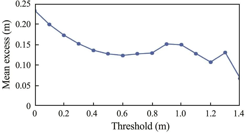
Fig.9 Mean excess of storm surges in the study region.

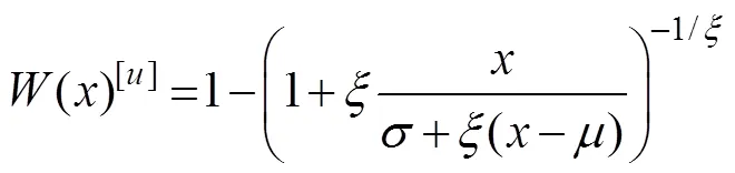
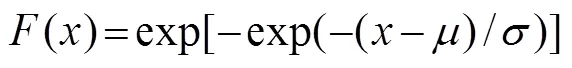
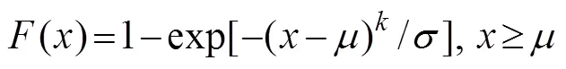
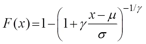
Four common extreme value distribution functions(Gum- bel, Weibull, GPD, and Pearson type III [P-III]) were selected to simulate storm surges that have longer return periods on the basis of the POT method. The distribution functions are expressed as follows:

Gumbel function:

Weibull function:

GPD function:

P-III function:

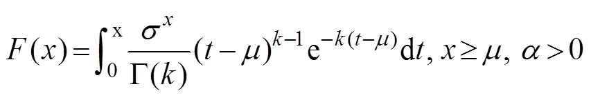
where,,anddenote the location, scale, and shape parameters in Eqs. (14)–(17), respectively.

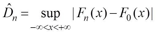
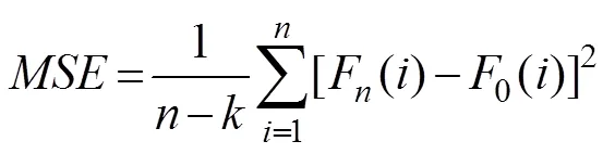
The fitting curve of each distribution function is shown in Fig.11. The goodness-of-fit test can identify how well the distribution of the hypothesized extreme values fits the actual empirical data on the basis of their calculated discrepancies. For this test, the following methods were applied:

Kolmogorov-Smirnov (-) test:

Mean squared error () method:

Akaike information criterion ():

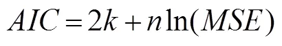
whereis the number of model parameters.

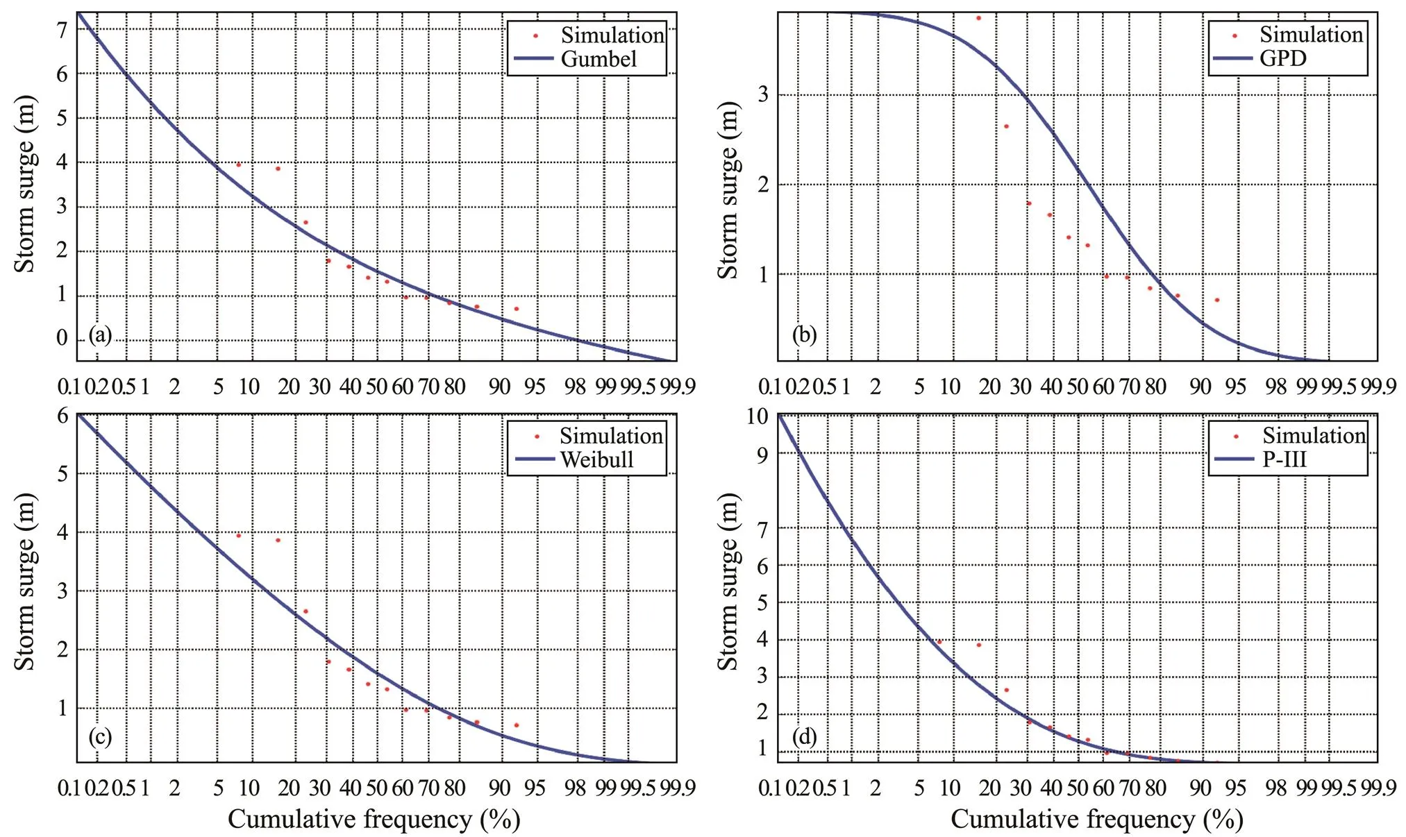
Fig.11 Fitting curves of storm surges based on the Gumbel, Weibull, GPD, and P-III distributions.

Table 2 Goodness-of-fit comparisons and estimated surges with different return periods based on different extreme value distributions

3.3 Mean Sea Level Rise

Sea level rise is a global-scale phenomenon caused by global warming, polar glacier melting, thermal expansion of the upper ocean, and other factors.Sea level rise caused by climate change poses a great threat to coastal areas, causing varying degrees of damage and loss.A review of the twentieth century by the Intergovernmental Panel on Climate Change states that global sea levels have risen by 10–20cm over the past 100 years (Church, 1991) at an average rate of approximately (1.8±0.1)mmyr?1(Douglas, 1991, 1997). Impact and risk assessment, adaptation policies, and long-term decision-making in coastal areas are crucially informed by projections of coastal mean sea leveland extreme water level events (Nicholls, 2014; Hin- kel, 2015; Kopp, 2017; Le Cozannet, 2017; Jevrejeva, 2018).Sea level rise has thus become an important global environmental problem that has been the subject of great attention from all sectors of society.

On the basis of the measured monthly mean sea level data for Chittagong between 2007 and 2016 (https://www.gloss-sealevel.org), a linear regression analysis wasconducted (Fig.12), which showed that the monthly mean sea level in Chittagong exhibits a rising trend at a rate of 0.0001m per month. This finding indicates that sea level rise around Chittagong has not necessarily been marked. On the basis of this rate of change, the sea level around Chittagong is expected to rise by 0.06 and 0.12m 50 and 100 years into the future, respectively.

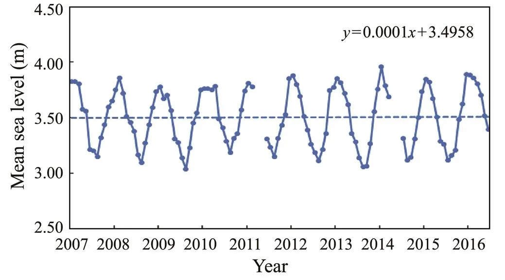
Fig.12 Linear regression analysis of monthly mean sea level data for Chittagong.

3.4 Inundation Assessment

During the calculation of flood extent, two cases should be distinguished, namely, the so-called nonsource flood and source flood, because each is based on different algorithms. In the case of a nonsource flood, all points with elevations below the given water level are included in the flooded area. This situation corresponds to the case of a well-distributed rainstorm over a large area where all low-lying land may be flooded. Alternatively, the source flood describes a flood pulse flushing through near-river regions,, as a result of a bank burst or where a smaller rainstorm causes localized flooding. The estimation of source floods needs to account for circulating conditions because only locations where the floodwaters can reach are inundated (Liu andLiu, 2002; Su, 2007). For storm surge flood- ing, floodwaters typically spread inland from an embankment; thus, the source flood model is most applicable.Furthermore, for a specific flood-control region, flooding can take two forms: overflowing flooding and dike-burst flood- ing.We consider only dike-burst flooding in this work, excluding the relationships between overflow mechanismsand dam structure, wind speed, and water depth at the foot of the embankment.

Storm surge flood routing with source flooding was adopted using a seed spread algorithm. This method involves selecting one or more representative pixels as a ‘seed’ that is given a particular set of attributes and then examining its contiguous pixels in four or eight outward directions. When contiguous pixels meet the specified conditions, they become further ‘seed’, and their contiguous pixels are examined in the same way, and so on. The pixels that meet the flood criteria are recorded cumulatively so that the resultant flooded area expands continuously. The process is repeated until all connected pixels have been examined according to the given conditions.

To determine the flood inundation extent, extreme sea levels were used as the fixed flood levels, and the location of storm surges served as the seed point, extending outwards in eight directions. According to the elevation data, if a storm surge height was greater than the elevation of a pixel, then it was included within the flooded area. The final flooded area for each scenario was then visualized on a raster map.This whole approach is presented schematically in Fig.13.

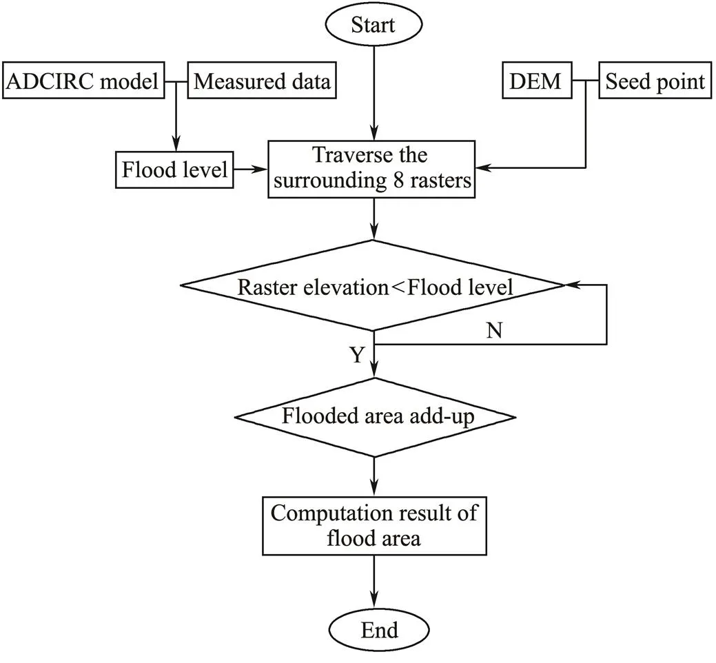
Fig.13 Flowchart schematic of the seed spread algorithm used to estimate flooding extent.

Four scenarios were designed to assess the risk of flooding in Chittagong, as shown in Table 3.Scenario 1 considered an extreme sea level resulting from the 50-year return period storm surge and a maximum astronomical high tide. Scenario 2 considered the 100-year return period storm surge and maximum astronomical high tide. These two scenarios did not consider the impact of sea level rise.Scenarios 3 and 4 were the same as Scenarios 1 and 2, but they also considered sea level rise after 50 and 100 years, respectively.

According to the hourly water-level data recorded at Chittagong Station from May to October 2007–2017, the maximum astronomical high tide water level was 3.15m.The simulations assumed that the peak storm surge water levels coincided with this astronomical high tide level, thus allowing us to estimate the flooding extent under extreme conditions.The maximum storm surge heights were 5.67 and 6.68m for the 50-year and 100-year return period, respectively, giving a combined maximum water level of 8.82 and 9.83m for Scenarios 1 and 2, respectively.With the inclusion of estimated sea level rises of 0.06 and 0.12m (Section 3.2, Table 3), maximum water levels of 8.89 and 9.97m were obtained for Scenarios 3 and 4, respectively.

The Chittagong water level station was used as the flood- ing seed point (91.825?E, 22.247?N).Fig.14 shows the esti- mated inundation depths for each scenario, and Fig.15 shows the floodwater propagation direction.Table 4 shows the maximum flooded areas under each scenario, which were 11.35, 36.44, 11.35, and 36.44km2, respectively.Notably, sea level rise had a minimal effect on the maximum flooded area, indicating that future sea level rise will have no clear impact on the inundation risk in Chittagong.As such, Scenarios 3 and 4 were not further considered.

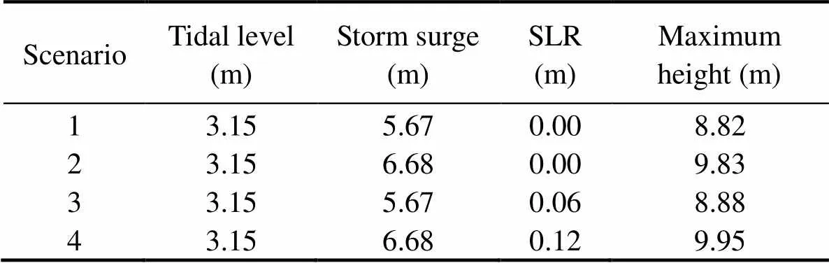
Table 3 Inundation model inputs for the four simulated scenarios

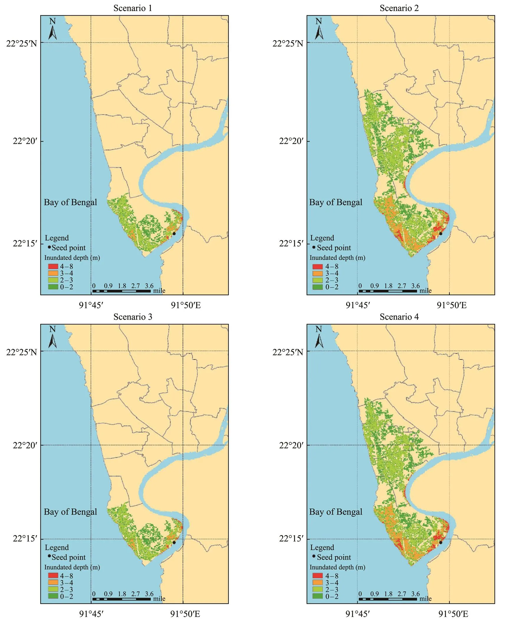
Fig.14 Submerged water depths in Chittagong under four different scenarios (see Table 4).

Fig.15 Floodwater propagation trends in Chittagong under four different scenarios (see Table 4).

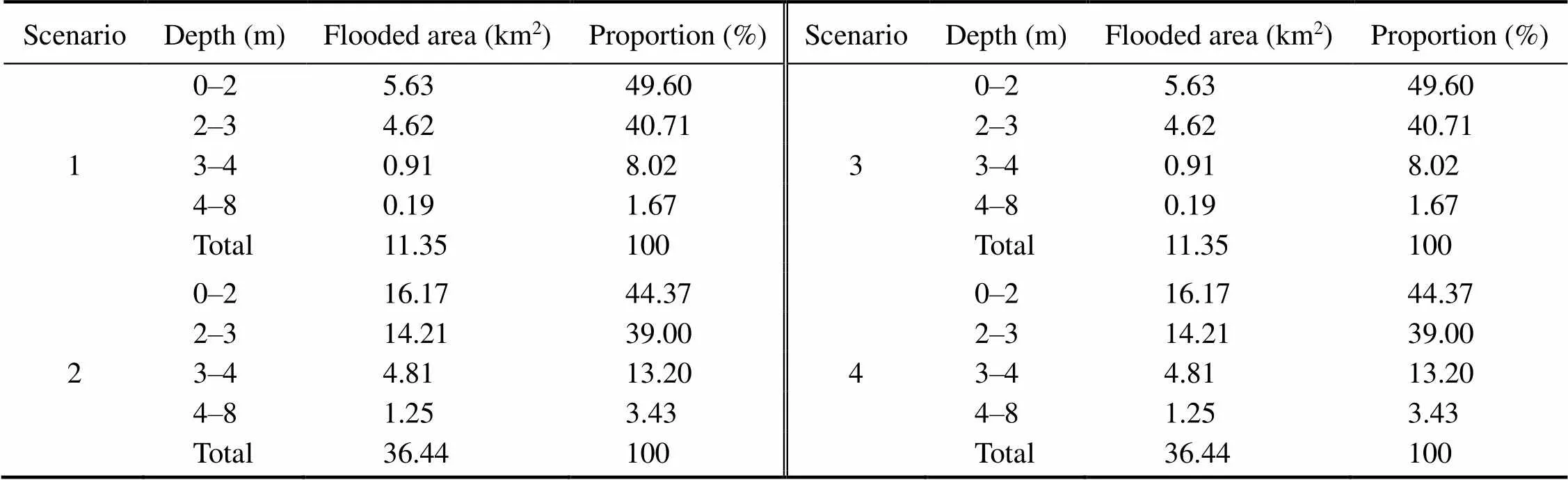
Table 4 Flooded area under each scenario inundation depth

On the basis of Fig.14, coastal areas are more vulnerable to flooding due to their low-lying terrain and are prone to having deeper floodwater depths.Under Scenarios 1 and 3, submerged water depths of 0–2m were predicted for an area of 5.63km2(accounting for 49.60% of the total flooded area); depths of 2–3m covered an area of 4.62km2(40.71%); depths of 3–4m covered an area of 0.91km2(8.02%); and depths of 4–8m covered 0.19km2(1.67%).Under Scenarios 2 and 4, submerged water depths in the range of 0–2m covered an area of 16.17km2(accounting for 44.37% of the total flooded area); depths of 2–3m covered 14.21km2(39.0%); depths of 3–4m covered 4.81km2(13.20%); and depths of 4–8m covered 1.25km2(3.43%).The difference in flooding extents between Scenarios 1 and 2 was 25.1km2, indicating that the difference in water levels between these two scenarios (, 1.01m) would result in a significantly greater inundation extent.

The floodwater propagation trends are illustrated in Fig.15. For Scenario 1, with a flood level of 8.82m, both the western coastal and southeastern river coastal plain areas are at risk of inundation due to their low-lying terrain.Thenortheast area of the city has a relatively high elevation (Fig.15a) and thus has a lower inundation risk.For all scenarios, flooding generally spreads from the southeast to the northwest.For Scenario 2, with a flood level of 9.83m, floodwaters spread further to the north, moving in a south–north direction, resulting in a larger inundation extent.Fig.15b shows that the terrain of the city is higher in the east and west and lower in the middle, allowing floodwaters to spread toward the north. Therefore, once flood levels reach the levels presented in Scenario 2, most areas in the north of the city are at risk of inundation.

4 Conclusions

The flood inundation risk of Chittagong was assessed under various storm surge disasterscenarios.Wind and pressure fields were constructed using the Jelesnianski typhoon model, and the ADCIRC hydrodynamic model was used to simulate astronomical tides and storm surges.The simulation results were verified using observation data, and they show that the model satisfactorily reproduced the astronomical tides and storm surge levels.The POT method and the P-III distribution function were used to evaluate the flood risks from 50-year and 100-year return period storm surges reaching levels of 5.67 and 6.68m, respectively.

For four scenarios, the flood inundation extent was determined using a DEM and a seed spread algorithm, and it was mapped using a GIS.The simulations accounted for the highest astronomical tide level, extreme storm surges, and sea level rise projections, giving combined maximum water levels of 8.82, 9.83, 8.89, and 9.97m, respectively.

The simulations showed insignificant effects of sea level rise on the inundation extent for Chittagong.At simulated flood levels of 8.82m (Scenario 1, 50-year storm surge without sea level rise) and 8.89m (Scenario 3, 50-year storm surge with sea level rise), the maximum flooded area was 11.35km2. Both the western and southeastern river coastal plain areas are at risk of flooding due to their low-lying terrain.Floodwaters generally propagated from the southeastern to the northwestern areas of the city. At flood levels of 9.83m (Scenario 2, 100-year storm surge without sea level rise) and 9.97m (Scenario 4, 100-year storm surge with sea level rise), the maximum flooded area was 36.4km2. Under these scenarios, floodwaters spread widely in the south–north direction, and most areas in the north of the city would be at risk of flooding.

Acknowledgements

This research was funded bythe National Key Research and Development Program of China (No. 2016YFC1401103), the Fundamental Research Funds for the Central Uni- versities (No. 202165003), and the Open Fund of Shandong Province Key Laboratory of Ocean Engineering, Ocean University of China (No. kloe201903).

Ali, A., 1979. Storm surges in the Bay of Bengal and some related problems. PhD thesis. University of Reading, England.

Arns, A., Wahl, T., Haigh, I. D., and Jensen, J., 2015. Determining return water levels at ungauged coastal sites: A case study for northern Germany., 65 (4): 539-554.

Bernardara, P., Andreewsky, M., and Benoit, M., 2011. Application of regional frequency analysis to the estimation of extreme storm surges., 116 (C2): C02008.

Bhaskaran, P. K., Gayathri, R., Murty, P. L. N., Bonthu, S., and Sen, D., 2014. A numerical study of coastal inundation and its validation for Thane cyclone in the Bay of Bengal., 83: 108-118.

Chittibabu, P., 1999. Development of storm surge prediction models for the Bay of Bengal and the Arabian Sea. PhD thesis. Indian Institute of Technology Delhi, New Delhi.

Choi, B. H., Kim, K. O., Yuk, J. H., and Lee, H. S., 2018. Simulation of the 1953 storm surge in the North Sea., 68: 1759-1777.

Church, J. A., Godfrey, J. S., Jackett, D. R., and McDougall, T. J., 1991. A model of sea level rise caused by ocean thermal expansion., 4 (4): 438-456.

Das, P. K., 1994. Prediction of storm surges in the Bay of Bengal., 60: 513-533.

Dietrich, J. C., Tanaka, S., Westerink, J. J., Dawson, C. N., Luettich Jr., R. A., Zijlema, M.,, 2012. Performance of the unstructured-mesh, SWAN?+?ADCIRC model in computing hurricane waves and surge., 52: 468-497.

Dietrich, J. C., Zijlema, M., Westerink, J. J., Holthuijsen, L. H., Dawson, C., Luettich Jr., R. A.,, 2011. Modeling hurricane waves and storm surge using integrally-coupled, scalable computations., 58 (1): 45-65.

Douglas, B. C., 1991. Global sea level rise., 96: 6981-6992.

Douglas, B. C., 1997. Global sea rise: A redetermination., 18: 279-292.

Dube, S. K., Jain, I., Rao, A. D., and Murty, T. S., 2009. Storm surge modelling for the Bay of Bengal and Arabian Sea., 51: 3-27.

Dube, S. K., Rao, A. D., Sinha, P. C., Murty, T. S., and Bahulayan, N., 1997. Storm surge in the Bay of Bengal and Arabian Sea: The problem and its prediction., 48 (2): 283-304.

Gonnert, G., Dube, S. K., Murty, T., and Siefert, W., 2001. Globalstorm surges: Theory, observations and applications., 623pp.

Gowri Shankar, C., Behera, M. R., and Vethamony, P., 2018. Sensitivity study of wind drag coefficient on surge modelling for tropical cyclone.. Springer, Singapore, 22: 813.

Hallegatte, S., Ranger, N., Mestre, O., Dumas, P., Corfee-Morlot, J., Herweijer, C.,, 2011. Assessing climate change impacts,sea level rise and storm surge risk in port cities: A case study on Copenhagen., 104 (1): 113-137.

Hatzikyriakou, A., and Lin, N., 2017. Simulating storm surge waves for structural vulnerability estimation and flood hazard mapping., 89: 939-962.

Hinkel, J., Jaeger, C., Nicholls, R. J., Lowe, J., Renn, O., and Shi, P. J., 2015. Sea-level rise scenarios and coastal risk management., 5: 188-190.

Jain, I., Rao, A. D., and Ramesh, K. J., 2010. Vulnerability assessment at village level due to tides, surges and wave setup., 33 (2-3): 245-260.

Jelesnianski, C. P., 1966. Numerical computations of storm surges without bottom stress., 94: 379-394.

Jevrejeva, S., Jackson, L. P., Grinsted, A., Lincke, D., and Marzeion, B., 2018. Flood damage costs under the sea level rise with warming of 1.5℃ and 2℃., 13 (7): 074014.

Kopp, R. E., DeConto, R. M., Bader, D. A., Hay, C. C., Horton, R. M., Kulp, S.,, 2017. Evolving understanding of Antarctic ice-sheet physics and ambiguity in probabilistic sea-level projections., 5 (12): 1217-1233.

Le Cozannet, G., Nicholls, R. J., Hinkel, J., Sweet, W. V., McInnes, K. L., Van de Wal, R. S. W.,, 2017. Sea level change and coastal climate services: The way forward., 5 (4): 49.

Le Provost, C., Bennett, A. F., and Cartwright, D. E., 1995. Ocean tides for and from TOPEX/POSEIDON., 267 (5198): 639-642.

Lewis, M. J., Palmer, T., Hashemi, R., Robins, P., Saulter, A., Brown, J.,, 2019. Wave-tide interaction modulates nearshore wave height., 69 (3): 367-384.

Liu, R. Y., and Liu, N., 2002. Flood area and damage estimation in Zhejiang, China, 66: 1-8.

Luettich Jr., R. A., Westerink, J. J., and Scheffner, N. W., 1992. ADCIRC: An advanced three-dimensional circulation model for shelves coasts and estuaries, report 1: Theory and methodology of ADCIRC-2DDI and ADCIRC-3DL. Dredging Research Program Technical Report DRP-92-6 US. Army Engineers Waterways Experiment Station, Vicksburg, MS, p137.

Murty, P. L. N., Sandhya, K. G., Bhaskaran, P. K., Jose, F., Ga- yathri, R., Nair, T. B.,, 2014. A coupled hydrodynamic modeling system for PHAILIN cyclone in the Bay of Bengal., 93: 71-81.

Murty, T. S., Flather, R. A., and Henry, R. F., 1986. The storm surge problem in the Bay of Bengal., 16: 195-233.

Nicholls, R. J., 2002. Analysis of global impacts of sea-level rise: A case study of flooding., 27: 1455-1466.

Nicholls, R. J., Hanson, S. E., Lowe, J. A., Warrick, R. A., Lu, X. F., and Long, A. J., 2014. Sea-level scenarios for evaluating coastalimpacts.,5: 129-150.

Nicholls, R. J., Hoozemans, F. M. J., and Marchand, M., 1999. In- creasingfloodriskandwetlandlossesduetoglobalsea-levelrise: Regionaland global analyses., 9: 69-87.

Pandey, S., and Rao, A. D., 2018. An improved cyclonic wind distribution for computation of storm surges., 92: 93-112.

Rao, A. D., 1982. Numerical storm surge prediction in India. PhD thesis. Indian Institute of Technology Delhi, New Delhi.

Rao, A. D., Jain, I., and Venkatesan, R. N., 2010. Estimation of extreme water levels due to cyclonic storms: A case study for Kalpakkam coast., 1 (1): 1-14.

Rao, A. D., Murty, P. L. N., Jain, I., Kankara, R. S., Dube, S. K., and Murty, T. S., 2013. Simulation of water levels and extent of coastal inundation due to a cyclonic storm along the east coast of India., 66 (3): 1431-1441.

Rao, A. D., Upadhaya, P., Pandey, S., and Poulose J., 2020. Sim- ulation of extreme water levels in response to tropical cyclones along the Indian coast: A climate change perspective., 100: 151-172.

Roy, G. D., 1984. Numerical storm surge prediction in Bangladesh. PhD thesis. Indian Institute of Technology Delhi, New Delhi.

Stuart, C., and Jonathan, T., 1991. Modelling extreme multivariate events., 53 (2): 377-392.

Su, G. Z., Li, Y., Liu, N., and Liu, R. Y., 2007. Visualization and damage assessment for flooded area., 7 (3): 180-186.

Tebaldi, C., Strauss, B. H., and Zervas, C. E., 2012. Modelling sea level rise impacts on storm surges along US coasts., 7 (1): 14-32.

Ubydul, H., Hashizume, M., Kolivras, K. N., Overgaard, H. J., Das, B., and Yamamoto, T., 2012. Reduced death rates from cyclones in Bangladesh: What more needs to be done., 90: 150-156.

Wang, Y. P., Liu, Y. L., Mao, X. Y., Chi, Y. T., and Jiang, W. S., 2019. Long-term variation of storm surge-associated waves in the Bohai Sea., 37: 1868-1878.

Wang, Z. F., Yu, M., Dong, S., Wu, K. J., and Gong, Y. J., 2020. Wind and wave climate characteristics and extreme parameters in the Bay of Bengal., 39 (15): 1-14.

Westerink, J. J., Blain, C. A., Luettich Jr., R. A., and Scheffner, N. W., 1994. ADCIRC: An advanced three-dimensional circulation model for shelves coasts and estuaries, Report 2: User’s manual for ADCIRC-2DDI. Dredging Research Program Tech- nical Report DRP-92-6, US Army Engineers Waterways Experiment Station, Vicksburg, MS, 156pp.

Zheng, L., Weisberg, R. H., Huang, Y., Luettich, R. A., Westerink, J. J., Kerr, P. C.,, 2013. Implications from the comparisons between two and three-dimensional model simulations of the Hurricane Ike storm surge., 118 (7): 3350-3369.

(January 9, 2022;

February 20, 2022;

April 6, 2022)

? Ocean University of China, Science Press and Springer-Verlag GmbH Germany 2023

. E-mail: lisongtao@ouc.edu.cn

(Edited by Xie Jun)