Elastic-Wave Reverse Time Migration Random Boundary-Noise Suppression Based on CycleGAN

XU Guohao, and HE Bingshou, *

Elastic-Wave Reverse Time Migration Random Boundary-Noise Suppression Based on CycleGAN

XU Guohao1), 2), and HE Bingshou1), 2), *

1),,266100,2),,266100,

In elastic-wave reverse-time migration (ERTM), the reverse-time reconstruction of source wavefield takes advantage of the computing power of GPU, avoids its disadvantages in disk-access efficiency and reading and writing of temporary files, and realizes the synchronous extrapolation of source and receiver wavefields. Among the existing source wavefield reverse-time reconstruction algorithms, the random boundary algorithm has been widely used in three-dimensional (3D) ERTM because it requires the least storage of temporary files and low-frequency disk access during reverse-time migration. However, the existing random boundary algorithm cannot completely destroy the coherence of the artificial boundary reflected wavefield. This random boundary reflected wavefield with a strong coherence would be enhanced in the cross-correlation image processing of reverse-time migration, resulting in noise and fictitious image in the migration results, which will reduce the signal-to-noise ratio and resolution of the migration section near the boundary. To overcome the above issues, we present an ERTM random boundary-noise suppression method based on generative adversarial networks. First, we use the Resnet network to construct the generator of CycleGAN, and the discriminator is constructed by using the PatchGAN network. Then, we use the gradient descent methods to train the network. We fix some parameters, update the other parameters, and iterate, alternate, and continuously optimize the generator and discriminator to achieve the Nash equilibrium state and obtain the best network structure. Finally, we apply this network to the process of reverse-time migration. The snapshot of noisy wavefield is regarded as a 2D matrix data picture, which is used for training, testing, noise suppression, and imaging. This method can identify the reflected signal in the wavefield, suppress the noise generated by the random boundary, and achieve denoising. Numerical examples show that the proposed method can significantly improve the imaging quality of ERTM.

random boundary; reverse-time migration; generative adversarial network; noise suppression

1 Introduction

In multi-component seismic exploration, the elastic-wave reverse-time migration (ERTM) (Chang and McMechan, 1987; Yan and Sava, 2008; Wang and McMechan, 2015) is an effective tool for P- and S-wave imaging. It mainly consists of three parts: 1) forward extrapolation of source wavefield, 2) reverse-time extrapolation of receiver wavefield, and 3) P- and S-wave imaging using cross-correlation imaging conditions. For the reduction of the amount of reading and writing of temporary files and improvementof the computational efficiency, a reverse-time reconstruction is needed after the forward extrapolation of the source wavefield to realize the synchronous extrapolation of the source and receiver wavefields. Simultaneously, the decoupling of P- and S-waves is necessary during source- wavefield reconstruction and receiver wavefield reverse- time extrapolation, which decouples the elastic source and receiver wavefields into the P- and S-wavefields at each time step, to attain migration results with evident physical meaning. In addition, for the suppression of the migration noise such as inter-layer reflection, the source and receiver wavefields need to be decomposed based on the propagation direction in the extrapolation process to obtain the P- and S-wave propagations in different directions, enabling the selection of the wavefield in a specific propagation di- rection to participate in the cross-correlation operation in subsequent imaging conditions (Duan and Sava, 2015).

The reverse-time reconstruction of source wavefields (Feng and Wang, 2012) in reverse-time migration is attri- buted to the reverse-time migration of elastic wave, which realizes the accurate P- and S-wave imaging through the correlation of the source and receiver wavefields; however, the construction of source and receiver wavefields is usually carried out in the opposite time direction, and the cross-correlation imaging conditions require that both have the same extrapolation sequence. This inconsistency will increase the disk access of reverse-time migration and reduce computational efficiency. Geophysicists often adoptthe strategy of ‘replacing storage with computation’ (Dussaud., 2008) to overcome the above issues, in particular, to carry out two source wavefield extrapolations, store part of the wavefield information during the first extrapolation, and use this information to reconstruct the source wavefield in reverse time after the extrapolation is completed. Meanwhile, the source wavefield is reconstruct- ed, and the reverse-time extrapolation of the receiver wave- field is executed at the same time to realize the synchronous extrapolation of the source and receiver wavefields and low-frequency disk access in the process of migration imaging.

At present, four strategies are used to realize sourcewavefield reverse-time reconstruction: 1) Source wavefieldreconstruction method based on checkpoint technology(Symes, 2007). The wavefield reconstruction accuracy de- pends on the number of checkpoints. An extremely low number of checkpoints cannot ensure reconstruction accuracy. Increasing the number of checkpoints will increase disk access. Simultaneously, the defect of high recalculation rate should be considered by this method. 2) Source- wavefield reverse-time reconstruction method based on boundary storage strategy (Clapp, 2009). The recalculation rate of this method is 2, and its temporary file storage ca- pacity mainly depends on the number of edge layers. The excessive number of edge layers will lead to the rapid in- crease of storage capacity. On the contrary, extremely few edge layers will increase the boundary reflection noise. 3) Reconstruction method based on effective boundary sto- rage strategy (Yang., 2014). This method is an impro- vement of the boundary storage strategy and only needs to store theth-layer boundary wavefield (is semi-diffe- rential order), and the recalculation rate is still 2. 4) Source-wavefield reconstruction method based on the randomboundary (Clapp, 2009). In this method, a layer with random elastic parameters is added outside the model to scatter the outward traveling wave in the boundary region to weaken the coherence of the boundary reflected wave and reduce the influence of the boundary reflected wave on the imaging. The recalculation rate is 2, with no requirement for disk reading and writing.

From the above analysis, among the existing reverse- time reconstruction techniques of source wavefield, the ran- dom boundary algorithm has the lowest recalculation rate and temporary file storage and can achieve the highest calculation efficiency. Therefore, the random boundary algo- rithm has become an important algorithm in the field of reverse-time migration.

The random boundary breaks the coherence of reflected wavefields at the boundary to scatter the traveling wave through a layer of random elastic parameters embedded outside the calculated boundary. The poorer the coherence of the scattered waves in the random layer, the less the effect of calculated boundaries on the migration results.Theoretically, the effect of boundary reflection on reverse- time migration is zero when the random layer thickness is sufficiently large and the randomness of elastic parameters sufficiently desirable. However, in the actual calculation, given the limited thickness of the random layer and the difficulty in assigning completely random elastic parameters to the media in the random layer, the scattered wavefields of the random boundary often present a certain coherence. Such boundary scattered wave with coherence is passed to the migration results by imaging conditions, resulting in noise in the reverse-time migration result. Con- sequently, mechanisms for the reduction of coherence of randomly scattered waves are a current research focus in the research field.

The rational construction of random elastic parameters is one of the ways to reduce the coherence of scattered waves of random layers, and numerous scholars have studied the construction of random boundaries. Clapp (2009) employed a linear random function to construct random boundaries. The method requires a large random layer thickness. Otherwise, a coherent reflection with strong energy will be formed in the outer layer of the boundary. Zhang and Cheng (2017) used a random medium expression described by three parameters, including auto-corre- lation function, correlation length, and standard deviation of velocity perturbation, to construct parametric random boundaries. The test results showed that the random medium with exponential autocorrelation function had a better scattering effect on the wavefield. Increasing the perturbation velocity can enhance the scattering effect of the wavefield, but the random boundary can achieve the best result when the correlation length is close to the wavelength, and the standard deviation of velocity perturbation is about 30% on the condition that the algorithm is stable.Clapp and Shen (2015) constructed random boundary by controlling the size and morphology of random velocity particles, and the findings showed that without increasing random boundary thickness, using large-scale random ve- locity particles can effectively scatter the low-frequency components of the wavefield and weaken the coherence of boundary reflected waves. However, when the random lay- er thickness is small, the boundary scattered wavefields still have strong coherence, which causes the migration re- sult to produce a coherent noise near the calculation boun- dary. Notably, an increasing random layer thickness can solve the problem to a certain extent to compensate for the cost of increasing memory demand and computation time.

In this paper, we present a method of random boundary noise suppression for ERTM based on the CycleGAN net- work. The noise at the random boundary of ERTM is different to a certain extent from the effective signal, and a remarkable feature of deep learning (Mauricio., 2018) is its capability to discover features hidden in high- dimensional data. Considering the noise generated by random boundary in wavefield snapshots as the identification feature, we set the CycleGAN network to automatically complete noise suppression in large quantities. The CycleGAN structure is trained by the training data set with noise and without noise. When the generator and discri- minator parameters are optimal, the training is stopped, and the optimal model is saved. The noisy wavefield snap-shots in the reverse-time reconstruction of the source wave- field are used to test the suppression of random noise. The test results are used for reverse-time migration imaging to obtain the PP migration and PS migration section. The migration results prove the effectiveness of the method in this paper.

2 Basic Principles of ERTM

ERTM is generally achieved by numerically solving the source and receiver wavefields of each imaging point and the cross-correlation between the source and receiver wave- fields using the principle of time consistency. For two-di- mensional cases, the reverse-time migration of elastic wave often employs a method similar to Eq. (1) for P- and S- wave imaging:

whereandare the spatial coordinates (m),maxis the record length (ms),pp(,,) is the PP migration section,ps(,,) is the PS migration section,(,,) is the source P-wave, and(,,) and(,,) are the receiver P- and S-waves, respectively.

The application of Eq. (1) to P- and S-wave imaging often produces a strong low-frequency noise in the migration result. This low-frequency noise is caused by the cross- correlation between the wavefields of the source and receiver in the same direction, which will seriously reduce the signal-to-noise ratio of the migration result. Thus, the noise must be suppressed in regard to its basic generation mechanism. The common noise suppression method is to decompose the wavefield by using the propagation direction of the wave before imaging, decompose it into P- and S-waves propagating in different directions, and then select only the wavefield in a specific propagation direction to participate in the cross-correlation operation during imaging to eliminate the migration noise. Therefore, the imaging conditions become the following:

In this paper, the imaging of P- and S-waves is carried out using Eq. (2), in which the propagation direction of waves is obtained from the Poynting vector (Yoon and Marfurt, 2006) of the elastic wavefield.

3 Random Boundary of ERTM and Its Migration Noise

Eqs. (1) or (2) requires using the same time sequence forthe extrapolation of source and receiver wavefields. However, in the actual calculation, the construction of source and receiver wavefields is often carried out in the opposite time direction, which increases the difficulty of realizing reverse-time migration. The intuitive solution is to obtain the source and receiver wavefield values simultaneously through frequent disk access. Without additional computation, this algorithm will reduce the execution efficiency of parallel programs because of frequent disk access. Therefore, the practical value of this algorithm is limited.

The industry adopts the concept of replacing storage withcalculation to reduce the storage of temporary files and the hard-disk reading and writing capacity. Specifically, two source wavefield extrapolations are executed. Stored partial wavefield information at the first extrapolation is used to reconstruct the source wavefield in reverse time. While reconstructing the source wavefield, the reverse-time extrapolation of the receiver wavefield is executed in parallel, realizing the synchronous extrapolation of the source and receiver wavefields. Thus, the storage of temporary files and frequent disk reading and writing in the process of reverse-time migration can be avoided, which can use the advantages of the computational power of parallel com- puters and improve migration efficiency.

Random boundary algorithm is an efficient source-wave- field reverse-time reconstruction method; it scatters the outward traveling wave in the boundary region by embed- ding a layer with random elastic parameters outside the model. Given that the random boundary algorithm does not need to split or attenuate the wavefield at the boundary, the wavefield propagation process based on the random boundary and finite difference is reversible. Therefore, the forward extrapolation algorithm of the source wavefield can be directly used for reverse-time reconstruction.

We use the above method to reconstruct the source wave-field and adopt Eq. (3) to assign the random velocity (Clapp, 2009) of P- and S-waves at the boundary:

whererandom(,) is the random velocity of P- or S-wave at point (,) in the boundary layer,(,) is the corresponding background velocity of P- or S-wave,is arandom number,is the distance between point (,) in the random boundary layer and the regional boundary, and0(,) is the maximum stable velocity, which is obtained from the stability condition (Zeng., 2001) of the finite difference of the elastic wave equation.

Figs.1(a) and 1(b) show the P- and S-wave velocity fields after embedding a random velocity layer outside the calculation space of uniform medium, in which the background velocities of P- and S-wave are 3000 and 1732ms?1, respectively. The accuracy of reverse-time reconstruction of the source wavefield at the random boundary is tested by this velocity model. During forward extrapolation, the P-wave excitation source is located at the center of the model, and the source wavelet is a Ricker wavelet with a dominant frequency of 30Hz. The difference lattice (Dablain, 1986) with 12th-order spatial accuracy and 2nd- order time accuracy is used for calculation in a staggered grid space. Figs.2(a) and 2(b) present two wavefield snapshots ofandcomponents, respectively, at 0.5s in the forward extrapolation process of the wavefields. Given that the P-wave excited by the source has not reached the boundary area at this time, the random boundary has no effect on the wavefield snapshots. We can consider this finding an accurate result without considering the error of the finite difference algorithm. Figs.3(a) and 3(b) show the two wavefield snapshots ofandcomponents, respectively, at 0.8s during the forward extrapolation of wave-fields. At this point, the P-wave excited by the source reach- es the boundary area. The random boundary layer plays a scattering role for the boundary reflections, but a coherent noise still exists. Figs.4(a) and 4(b) display two wavefield snapshots of theandcomponents, respectively, after the wavefield extrapolation at 3s. At this point, given that the direct wave excited by the source has completely pass- ed through the whole calculation area, disorderedly scattered waves remain in the wavefield snapshots of the two- component.

With the snapshots shown in Fig.4 as the initial condition, the source wavefield is reversely reconstructed using the same difference format. Figs.5(a) and 5(b) show theandcomponent wavefield snapshots, respectively, at 0.8 s after reconstruction. The reconstructed wavefield snapshot shows a slight difference with the forward extrapolation, which indicates that the random boundary algorithm can realize the accurate reverse-time reconstruction of the source wavefield. However, the drawback of the random boundary algorithm is that given the limited thickness of the random layer and the cannot be completely random ela- stic parameters, the scattered waves generated by the random layer still have a certain coherence, resulting in an evident noise in the calculation area near the boundary (most of the energy in Figs.3 and 5 belong to this noise). When this noisy wavefield is substituted into Eq. (2) for imaging, a remarkable migration noise will be generated in the area close to the boundary.

Fig.1 P- and S-wave velocities at the random boundary of a two-dimensional uniform medium. (a), P-wave velocity field; (b), S-wave velocity field.

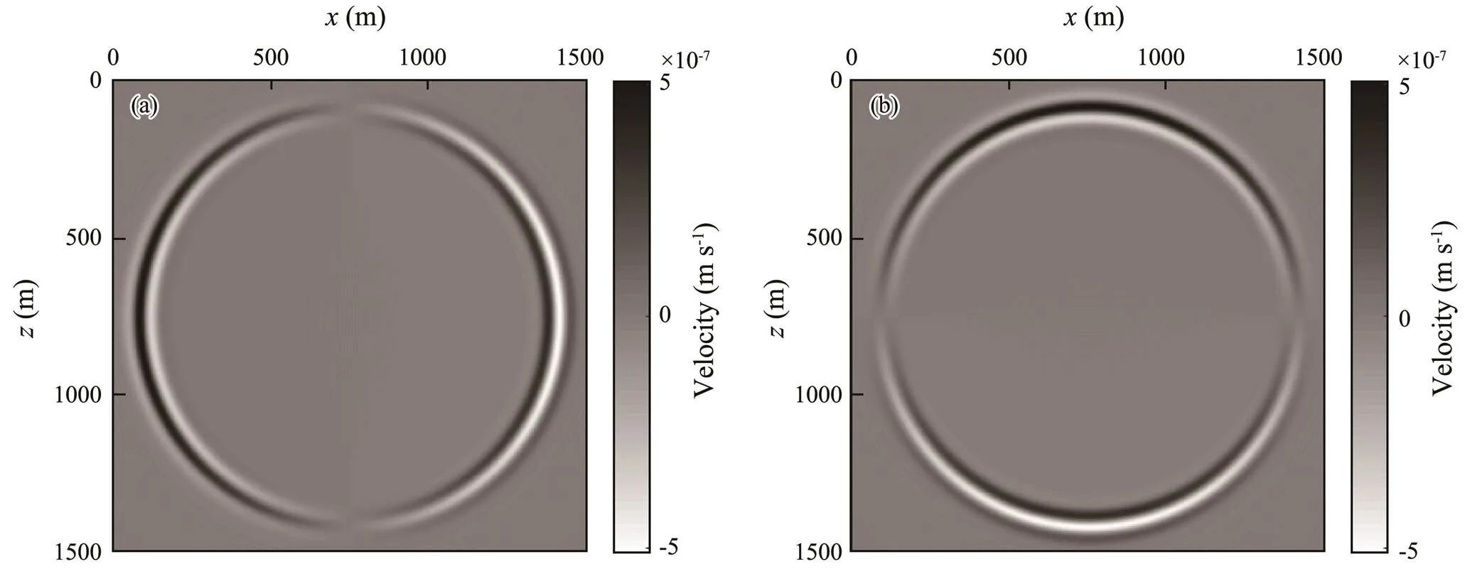
Fig.2 Wavefield snapshots of forward extrapolation at the random boundary in a two-dimensional uniform medium at 0.5s. (a), vx component; (b), vz component.

Fig.3 Wavefield snapshots of forward extrapolation at the random boundary in a two-dimensional uniform medium at 0.8s. (a), vx component; (b), vz component.

Fig.4 Wavefield snapshots of forward extrapolation at the random boundary in a two-dimensional uniform medium at 3.0s. (a), vx component; (b), vz component.

Given a two-layer model with one horizontal reflection interface as an example, the influence of random boundarynoise on the migration section is analyzed. The model size is 1500m×1500m, and the buried depth of the reflection interface is 750m. The P- and S-wave velocities are 3000 and 1732ms?1, respectively, and the density of the first lay- er of the medium equals 2100gcm?3. For the second layer,the P- and S-wave velocities are 3500 and 2000ms?1, respectively, and the density is 2500gcm?3, respectively. Themodel is forward modeled (Virieux, 1984) by the 2nd-ordertime and 12th-order spatial precision finite difference me- thod (Dong., 2000). The observation system used for forward modeling is the dominant frequency of a 30Hz Ricker wavelet source placed at 750 and 0m, the P-wave source, and 300 channels receiver located on the surface (from 0m to 1500m) with an interval of 5m. The forward modeling parameters are as follows: square grid division, space step size of 5m, time division step size of 0.5ms, and record length of 3s. The random boundary algorithm is used for reverse-time migration of the two-component synthetic seismic records obtained by forward modeling. Figs.6(a) and 6(b) show the PP and PS migration results of single-shot records by random boundary algorithm, respectively. Figs.7(a) and 7(b) present the PP and PS migration results of single-shot records by disk-access algorithm, respectively. Fig.6 reveals a shallow migration noise caused by scattering noise of the random boundary, which will reduce the imaging accuracy of reverse-time migration for shallow formation. Meanwhile, Fig.7 shows no re- markable shallow migration noise. Therefore, appropriate technologies must be used to eliminate this noise.

Fig.5 Snapshots of the reconstructed wavefield at the random boundary in a two-dimensional uniform medium at 0.8s. (a), vx component; (b), vz component.

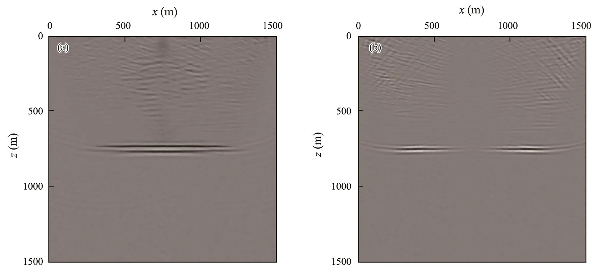
Fig.6 Single-shot migration section of the horizontally layered model by the random boundary algorithm. (a), PP migration section; (b), PS migration section.

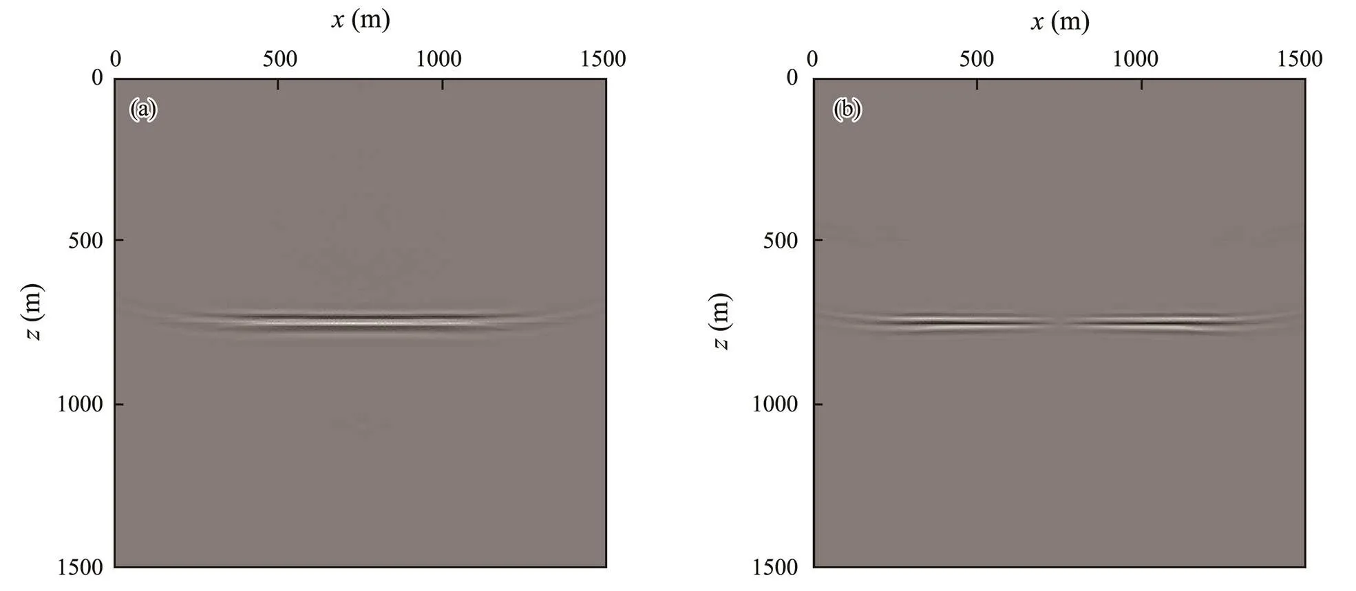
Fig.7 Single-shot migration section of the horizontally layered model by the disk-access algorithm. (a), PP migration section; (b), PS migration section.

4 Suppression Methods

4.1 Principle of Generative Adversarial Networks (GANs)

The basic idea of GANs (Goodfellow., 2014) ori- ginates from the ‘zero-sum game’ in game theory, which means that the sum of gains and losses of the two parts in a game is constantly zero. In this paper, the two parts involved in the game are generators and discriminators. The generator generates a sample() that obeys the real data distributiondata(a)through the input data. The function of the discriminator is to judge whether the input sample is a real sampleor a generated sample(). Generatorand discriminatorare trained alternately to train the optimization model through adversarial learning to achieve Nash equilibrium (Ratliff., 2006) and optimize the model parameters.

CycleGAN (Zhu., 2017) is composed of two mirrored symmetrical GANs. The model can realize the mu-tual transformation (Song, 2020) of two types of correlated samples and obtain the best mapping of the two types of sample space through adversarial learning. Compared with traditional GAN, CycleGAN has two improvements. 1) The input data can be unpaired training data, and the con- version from input data to target data can be realized without establishing a one-to-one correspondence between training data. 2) The cycle consistency loss function is introduced to strengthen the training process.

The specific composition is as follows: The CycleGAN network structure is composed of two GANs and constitutes a ring network (Dong., 2021). The network shares two generators (GandG) and has two discriminators (DandD) corresponding to them. The adversarial learning between generatorand discriminatorwill produce an adversarial loss. One-way GAN hasandlosses, whereas the two GANs of the CycleGAN network have two groups of adversarial losses ofDandG;DandG. The two groups of adversarial loss functions are as follows:

However, the training process of GAN is unstable and prone to generating only one specific datum in the target domain. Based on adversarial losses, CycleGAN uses cycleconsistency losses (Kaneko and Kameoka, 2018) as a constraint to avoid the conversion of all data in the domain to some data in another domain by the two generators of GAN; as a result, the generated data are consistent with the input itself as much as possible. The cycle consistency loss function is expressed as follows:

In Eq. (6),cyc(G,G) is the loss of cycle consistency function for generatorsGandG, andG(G()) andG(G()) are the data generated by the two generators for real sampleand input data, respectively.Thus, the total loss function can be obtained.

The total loss function of the CycleGAN network is the sum of two adversarial losses and one loss of cycle consistency:

In Eq. (7),total(D, D, G, G) is the total loss function for the entire CycleGAN.

The total loss function incorporates the adversarial loss and loss of cycle consistency, which results in close pro- ximity of the generated data to the real data and prevents the two generators from generating data that are in conflict with each other.

4.2 CycleGAN Network Structure

In the ERTM process, the reconstructed source wavefield is composed of the effective signal and the coherent noise at the boundary. The data characteristics of the effective signal and the coherent noise in the wavefield are notably different. Thus, relevant methods can be used to suppress the noise. The noise suppression method aims to obtain pseudo noiseless data by processing the snapshot ofthe noise-containing wavefield, and as a result, the pseudo noiseless data are close to the real noiseless data. Deep learning can extract statistical features of data and model any type of data distribution (Mauricio., 2018), accurately obtain data closer to the effective signal, and achieve good effects for more complex noise distribution.

In this paper, a CycleGAN network is used to suppress the noise generated by a random boundary in the wavefield snapshot. The CycleGAN algorithm needs to set up a suitable training set to train the data. In this problem, the training set is the snapshots of P- and S-waves with and without the noise of various geological models and wavefield snapshots after inversion and interpolation. The number of training samples with and without noise is 2700.

The concrete implementation is as follows. First, we determine sample spacesand,withandbeing the noisy and noiseless wavefield snapshots, respectively. Sec- ond, we determine the training parameters, including generator parameters, discriminator parameters, sample number, and iteration number. Then, iteration begins, and the optimal network structure is obtained by iterating and updating the parameters of the generator and discriminator. The iteration process is as follows: First, we selectsamples with the noise from sample spaceand generatepseudo noiseless samples from generatorG. Next, we selectnoiseless samples from sample spaceand ge- neratepseudo noise samples from generatorG. Then, the pseudo noiseless samples and noiseless samples are discriminated by discriminatorD, and a set of adversarial losses is obtained. The pseudo noise samples and noise samples are discriminated by discriminatorD, and another set of adversarial loss is obtained, from which the discri- minator parameters are updated. Finally, the pseudo noise samples generated by generatorsGandGand the pseu- do noiseless samples generated by generatorsGandGare obtained and compared with the noise and noiseless samples in the original sample space to obtain the cycle consistency loss. We then update the generator parameters again and proceed to the next iteration. Fig.8 shows the structure of the CycleGAN network.

During the actual training, the generator is prone to the generation of specific data, at which point the generator no longer updates its parameters, learning cannot be continued, and model training crashes. The CycleGAN network structure is used with a cache test to solve the instability problem during model training and further improve the stability of network training (Shrivastava., 2017). When updating the generator and discriminator parameters, the data generated before the interval time is adopted instead of the newly generated data nearby,., the historical data generated by buffer storage are adopted for later use.

4.3 Generator and Discriminator Selection

We use the Resnet network to build the generators of CycleGAN (Fig.9). The generator structure is as follows. First, the input data are a random noise-containing sample, which is convoluted using 64 convolution kernels (Conv) of size 7×7. Subsequent batch normalization (BN) allows the convolution-processed feature matrix to meet the specific distribution law, and the ReLU activation function is introduced to accept the output value of the previous neuron, served as the input value of the present unit, and passed on to the next neuron. Down-sampling is performed to obtain a new sequence and enter the Resnet network consisting of 6 residual blocks. Fig.10 shows the Resnet basicunit. The network is designed as()=()+to avoid directly fitting the identity map()=. The problem is transformed into finding the residual function()=()–, which constitutes a map()=if()=0. Fitting residuals is easier than directly fitting identity maps. Finally, after up-sampling, the data features are enlarged by interpolation, and 64 Conv with a size of 7×7 are used for con- volution. The tanactivation function is used as an input to connect the output of upper-layer neurons with that of lower-layer neurons, outputting the generated data.

Fig.8 CycleGAN structural diagram.

Fig.9 Random noise suppression by the CycleGAN generator

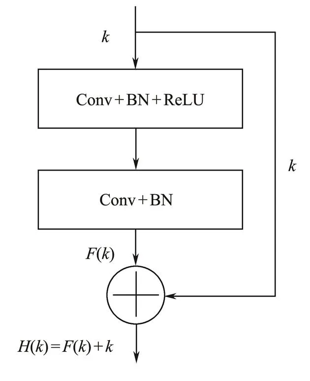
Fig.10 Resnet base unit.

Discriminator (Fig.11) uses the PatchGAN network. The traditional GAN outputs a real number as a discriminant result of the input data, whereas the PatchGAN network outputs a matrix (Yue., 2021) in which each element represents the discriminant result of that element on the corresponding input data. The input data of the net- work are noiseless and pseudo noiseless samples. After processing the convolution layers, which use 64, 128, 256, and 512 Conv with a size of 4×4, BN, and a leaky ReLU activation function with a slope of 0.2, which is used to connect the previous neuron output to the next, the noiseless and pseudo noiseless samples are turned into a 30 by 30 matrix.

Fig.11 Random noise suppression by the CycleGAN discriminator.

5 Effect Verification

The effectiveness of the algorithm in this paper is verified using the two-layer horizontal layered medium model corresponding to Fig.6. Keeping the approach of wavefield extrapolation and P- and S-waves imaging constant during the reserve-time course, we only insert the previously trained CycleGAN network model during the reverse-time reconstruction of the source wavefield and use this network to filter the two-component snapshots at eachtime step after reconstruction to eliminate the noise gene- rated by the random boundary. Figs.12(a) and 12(b) show the final results of the PP and PS migrations, respectively. Compared with Fig.6, the findings reveal that the method of this paper can suppress the shallow migration noise generated by the random boundary well.

Fig.12 Single-shot migration section of the horizontally layered model after denoising the CycleGAN network. (a), PP migration section; (b), PS migration section.

The model shown in Fig.13(a), which is a two-dimen- sional model drawn from the SEG/EAEG salt-dome P- wave model, is used to further verify the efficiency of the algorithm in this paper. The S-wave velocity of the two- dimensional model is obtained by dividing the P-wave velocity by 1.73, and the S-wave velocity is shown in Fig.13 (b). The single-shot records used for migration are obtainedby finite-difference forward modeling with 12th-order spaceand 2nd-order time accuracy. The observation system usedfor forward modeling is as follows: ground P-wave source excitation, Ricker wavelet with the main frequency of 30 Hz, shot interval of 15m, first shot point at the horizontal position of 0m, receiver in full array, channel interval of 15m, sampling interval of 0.0005s, and single-shot record length of 2.5s. A total of 225 two-component seismic re- cords are obtained. Figs.14(a) and 14(b) show the results of employing the conventional ERTM algorithm. Either PP or PS section exhibits numerous false seismic events and noise in the shallow sections of the figure, reducing the imaging effect. Figs.15(a) and 15(b) display the PP and PS migration sections obtained by employing the CycleGANalgorithm, respectively. Notably, the algorithm in this paperachieves an effective suppression of random boundary noise and improves the imaging accuracy for superficial strata.

6 Conclusions

The random boundary algorithm in ERTM can synchro- nously extrapolate the source and receiver wavefields and improve the efficiency of reverse-time migration because of low-frequency disk access during ERTM. Aiming at the issue of imaging accuracy of shallow strata caused by the noise generated from the random boundary, we propose a random-boundary noise suppression method based on CycleGAN under the condition of ERTM. Random-boun- dary noise suppression is achieved by constructing and optimizing the generators and discriminators of the CycleGAN denoised network to obtain the best network structure, and this network is applied to the reverse-time migration procedure. Studies have shown that the CycleGAN network-based denoising method can achieve the effective suppression of random boundary noise and improve the imaging of superficial strata of the ERTM. Nevertheless, the neural network depends on the appropriate training set. A process for obtaining the optimal training set and its application to complex practical data are worthy of further discussion and research.

Fig.13 P- and S-wave velocities of the salt-dome model. (a), P-wave velocity of the salt-dome model; (b), S-wave velocity of the salt-dome model.

Fig.14 Stack-migration section from the random-boundary ERTM. (a), PP stack-migration section; (b), PS stack migration section.

Fig.15 Stack-migration section after noise suppression by the CycleGAN network. (a), PP stack-migration section; (b), PS stack-migration section.

Acknowledgements

The study is supported by the National Natural Science Foundation of China (No. 41674118) and the Fundamental Research Funds for the Central Universities of China (No. 201964017).

Chang, W., and Mcmechan, G. A., 1987. Elastic reverse-time migration., 52 (10): 243-256, DOI: 10.1190/1.14 42249.

Clapp, R. G., 2009. Reverse time migration with random boundaries.. Houston, 1-10, DOI:10.1190/1.3255432.

Clapp, R. G., and Shen, X. K., 2015. Random boundary condition for memory-efficient waveform inversion gradient computation., 80 (6): R351-R359.

Dablain, M. A., 1986. The application of high-order differencing to the scalar wave equation., 51 (1): 54, DOI: 10. 1190/1.1442040.

Dellinger, J., and Etgen, J., 1990. Wave-field separation in two- dimensional anisotropic media., 55 (7): 914, DOI: 10.1190/1.1442906.

Dong, J. J., Tang, J., Zhou, R. Z., and Yang, C. Y., 2021. Research on adaptive denoising of one-dimensional time-varyingsignal based on cyclic generation countermeasure network., 50 (5): 10-12 (in Chinese with English abstract).

Dong, L. G., Ma, Z. T., and Cao, J. Z., 2000. Stability of the staggered-grid high-order difference method for first-order ela- stic wave equation., 43 (6): 904- 913, DOI: 10.1002/cjg2.107.

Duan, Y., and Sava, P., 2015. Scalar imaging condition for elastic reverse time migration., 80 (4): S127-S136, DOI: 10.1190/geo2014-0453.1.

Dussaud, E., Symes, W. W., Williamson, P., Lemaistre, L., and Cherrett, A., 2008. Computational strategies for reverse-time migration.. Vegas, 2267-2271.

Feng, B., and Wang, H. Z., 2012. Reverse time migration with source wavefield reconstruction strategy., 9 (1): 69-74.

Goodfellow, I. J., Pouget-Abadie, J., Mirza, M., Xu, B., Warde- Farley, D., Ozair, S.,, 2014. Generative adversarial networks., 27: 2672-2680, DOI: 10.1145/3422622.

Kaneko, T., and Kameoka, H., 2018. CycleGAN-VC: Non-pa- rallel voice conversion using cycle-consistent adversarial networks.. Rome, 2100-2140, DOI: 10.23919/EUSIPCO.2018. 8553236.

Mauricio, A., Joseph, J., Amir, A., and Taylor, D., 2018. Deep- learning tomography., 37 (1): 58-66, DOI: 10.1190/tle37010058.1.

McMechan, G. A., 1983. Migration by extrapolation of time-de- pendent boundary values., 31 (3): 413-420.

Ratliff, L. J., Burden, S. A., and Sastry, S. S., 2006. Characteri zation and computation of local Nash equilibria in continuous games.. Monticello, 917- 924, DOI: 10.1109/Allerton.2013.6736623.

Shrivastava, A., Pfister, T., Tuzel, O., Susskind, J., Wang, W. D., and Webb, R., 2017. Learning from simulated and unsupervised images through adversarial training.. Honolulu, 2242-2251, DOI: 10.1109/CVPR.2017.241.

Song, J., 2020. Binary generative adversarial networks for image retrieval., 128: 2243-2264.

Symes, W. W., 2007. Reverse time migration with optimal check- pointing., 72 (5): 213-221.

Tang, C., and Mcmechan, G. A., 2018. Elastic reverse time migration with a combination of scalar and vector imaging conditions.2018. Anaheim, 4453-4457, DOI: 10.1190/segam2018-2998139.1.

Virieux, J., 1984. SH-wave propagation in heterogeneous media: Velocity-stress finite-difference method., 51 (4): 265, DOI: 10.1071/EG984265a.

Wang, W. L., and McMechan, G. A., 2015. Vector-based elastic reverse time migration., 80 (6): S245-S258, DOI: 10.1190/geo2014-0620.1.

Wang, W. L., McMechan, G. A., and Zhang, Q. S., 2015. Comparison of two algorithms for isotropic elastic P and S vector decomposition., 80 (4): T147-T160, DOI: 10.119 0/geo2014-0563.1.

Yan, J., and Sava, P., 2008. Isotropic angle-domain elastic reverse-time migration., 73 (6): S229-S239, DOI: 10.1190/ 1.2981241.

Yang, P., Gao, J., and Wang, B., 2014. RTM using effective boun- dary saving: A staggered grid GPU implementation., 68: 64-72.

Yoon, K., and Marfurt, K. J., 2006. Reverse-time migration using the poynting vector., 37 (1): 102-106.

Yue, P., Dechang, P., Junfu, C., and Han, M., 2021. FDPPGAN: Remote sensing image fusion based on deep perceptual patchGAN., 33 (15): 1-17, DOI: 10.1007/S00521-021-05724-1.

Zeng, Y. Q., He, J. Q., and Liu, Q. H., 2001. The application of the perfectly matched layer in numerical modeling of wave propagation in poroelastic media., 66 (4): 1258- 1266, DOI: 10.1190/1.1487073.

Zhang, L. M., and Cheng, G., 2017. Random boundary conditions for parameter combination optimization and its application in seismic RTM., 41 (5): 890-898 (in Chinese with English abstract).

Zhu, H. J., 2017. Elastic wavefield separation based on the Helm- holtz decomposition., 82 (2): S173-S183, DOI: 10. 1190/geo2016-0419.1.

Zhu, J. Y., Park, T., Isola, P., and Efros, A. A., 2017. Unpaired image-to-image translation using cycle-consistent adversarial networks.. Venice, 2242-2251, DOI: 10.1109/ICCV.2017. 244.

August 24, 2021;

November 25, 2021;

January 5, 2022

? Ocean University of China, Science Press and Springer-Verlag GmbH Germany 2022

. Tel: 0086-532-66782297

E-mail: hebinshou@ouc.edu.cn

(Edited by Chen Wenwen)