
NUMERICAL ANALYSIS FOR VOLTERRA INTEGRAL EQUATION WITH TWO KINDS OF DELAY?
2019-05-31 03:39:26WeishanZHENG鄭偉珊
關(guān)鍵詞:艷萍
Weishan ZHENG(鄭偉珊)
College of Mathematics and Statistics,Hanshan Normal University,Chaozhou 521041,China E-mail:weishanzheng@yeah.net
Yanping CHEN(陳艷萍)?
School of Mathematical Sciences,South China Normal University,Guangzhou 510631,China E-mail:yanpingchen@scnu.edu.cn
Abstract In this article,we study the Volterra integral equations with two kinds of delay that are proportional delay and nonproportional delay.We mainly use Chebyshev spectral collocation method to analyze them.First,we use variable transformation to transform the equation into an new equation which is de fined in[?1,1].Then,with the help of Gronwall inequality and some other lemmas,we provide a rigorous error analysis for the proposed method,which shows that the numerical error decay exponentially in L∞ and L2ωc-norm.In the end,we give numerical test to con firm the conclusion.
Key words Volterra integral equation;proportional delay;nonproportional delay;linear transformation;Chebyshev spectral-collocation method;Gronwall inequality
1 Introduction
In this article,we consider the Volterra integral equation(VIE)with the proportional delay and the nonproportional delay

where the unknown function y(τ)is de fined on[0,T],T<+∞,and q is constant with 0
This theory of the Volterra integral equation played an important role in many disciplines.It arises in many areas,such as the Mechanical problems of physics,the movement of celestial bodies problems of astronomy,and the problem of biological population original state changes.It is also applied to network reservoir,storage system,material accumulation,etc.,and solve a lot problems from mathematical models of population statistics,viscoelastic materials,and insurance abstracted.The Volterra integral equation with proportional and nonproportional is one of the important part of Volterra integral equations.It has great signi ficance.Not only can it promote the development of integral equation and enrich integral equation theory,but also can improve the computational efficiency.There were many methods to solve Volterra integral equations,such as Legendre spectral-collocation method[1],Jacobi spectral-collocation method[2],spectral Galerkin method[3,4],Chebyshev spectral-collocation method[5,6]and so on.In this article,according to[5,6],we are going to use a Chebyshev spectral-collocation to deal with the Volterra integral equation with proportional delay and nonproportional delay.A rigorous error analysis is provided for the approximate solution that theoretically justi fies the spectral rate of convergence.Numerical test is also presented to verify the theoretical result.
We organize this article as follows.In Section 2,we introduce some spaces,some lemmas,and the Chebyshev collocation method,which are important for the derivation of the main result.In Section 3,the convergence analysis is carried out and Section 4 contains numerical test which is given to con firm the theoretical result.
Throughout this article,C denotes a positive constant that is independent of N,but depends on q,T and the given functions.
2 A Chebyshev Spectral Collocation Method
In this section,we first review Chebyshev spectral-collocation method.To this end,we begin with introducing some useful results preparing for the error analysis.

with the norm
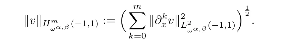
But in bounding the approximation error,only some of the L2-norms appearing on the righthand side of the above norm enter into play.Thus,for a nonnegative integer N,it is convenient to introduce the semi-norm

Particularly,when α = β =0,we denoteby Hm;N(?1,1).Whenwe denote
And the space L∞(?1,1)is the Banach space of the measurable functions u:(?1,1)→ R,which are bounded outside of a set of measure zero,equipped the norm

Next,we will give some lemmas,which are important for the derivation of the main results in the subsequent section.
Lemma 2.1(see[2,7]) Let Fj(x),j=0,1,···N,be the j-th Lagrange interpolation polynomials associated with N+1-point Chebyshev Gauss,or Chebyshev Gauss-Radau,or Chebyshev Gauss-Lobatto pointsThen,

where INis the interpolation operater associated with the N+1-point Chebyshev Gauss,or Chebyshev Gauss-Radau,or Chebyshev Gauss-Lobatto points,and promptly,

Lemma 2.2(see[1,8])Assume that,m>1,then the following estimates hold

Lemma 2.3(see[1,8])Suppose that,v ∈ Hm(?1,1)for some m>1 and ψ∈PN,which denotes the space of all polynomials of degree not exceeding N.Then,there exists a constant C independent of N such that
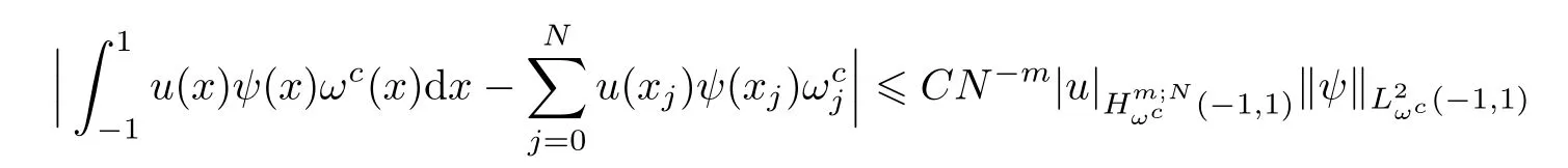
and

where xjis the N+1-point Chebyshev Gauss,or Chebyshev Gauss-Radau,or Chebyshev Gauss-Lobatto point,corresponding weight,j=0,1,···N and zjis N+1-point Legendre Gauss,or Legendre Gauss-Radau,or Legendre Gauss-Lobatto point,corresponding weight ωj,j=0,1,···N.
Lemma 2.4(see[9,10]Gronwall inequality) Assume that u(x)is a nonnegative,locally integrable function de fined on[?1,1],satisfying

where L≥0 is a constant and v(x)is an integrable function.Then,there exists a constant C such that

and

Lemma 2.5(see[11]) For all measurable function f>0,the following generalized Hardy’s inequality holds if and only if

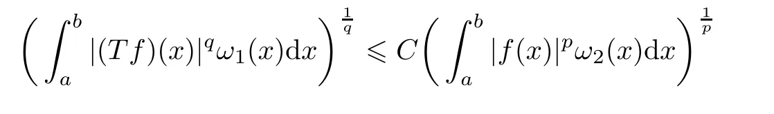
for the case 1

with k(x,t)being a given kernel,ω1,ω2weight functions,and ?∞6 a
Lemma 2.6(see[11,12]) For all bounded function v(x),there exists a constant C independent of v such that

Now,we describe the Chebyshev collocation method.We first use the variables transformation as follows

After that,(1.1)can be written as

where

Set the collocation points as the set of N+1-point Chebyshev Gauss,or Chebyshev Gauss-Radau,or Chebyshev Gauss-Lobatto points,(see,for examples[1]).Let xisubstitute in equation(2.1)and we have

To compute the integral term in(2.2)accurately,we transfer the integral intervals into a fixed interval[?1,1]by the following two simple linear transformations
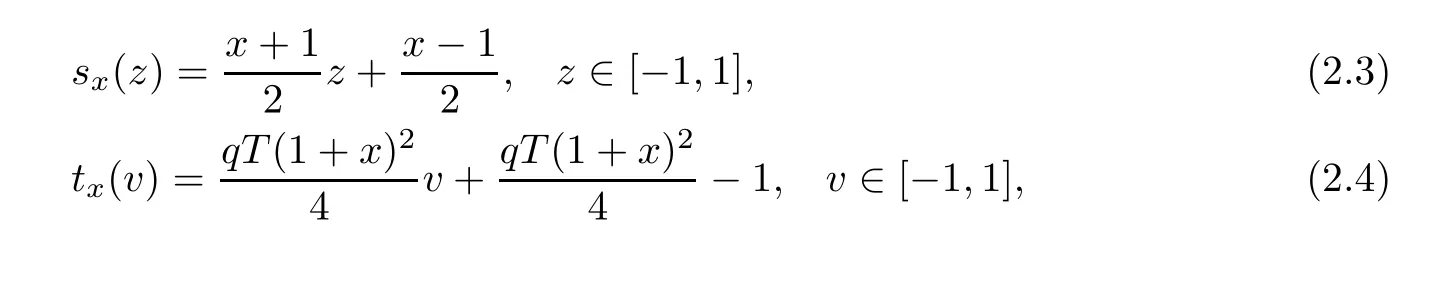
and then(2.2)becomes

here i=0,1,···,N,and

Next,using a N+1-point Gauss quadrature formula gives

for i=0,1,···,N,where zk=vkare the N+1-point Legendre Gauss,or Legendre Gauss-Radau,or Legendre Gauss-Lobatto points,corresponding weight wk,k=0,1,···,N(see,for example,[1]).We use uito approximate the function value u(xi)and use

to approximate the function u(x),where Fj(x)is the j-th Lagrange basic function associated withThen,the Chebyshev spectral-collocation method is to seek uN(x)such thatsatis fies the following equations for i=0,1,···,N,

We can also write the above equations in matrix form:U=G+AU,where

3 Error Analysis
This section is devoted to the analysis of convergence for equation(2.2).The goal is to show that the rate of convergence is exponential and the spectral accuracy can be obtained in L∞andspaces by using Chebyshev spectral-collocation method.First,we carry out the analysis in L∞space.
3.1 Error Analysis in L∞Space
Theorem 3.1Assume that u(x)is the exact solution to(2.1)and uN(x)is the approximate solution achieved by using the Chebyshev spectral collocation from(2.7).Then,for N sufficiently large,we get

where

ProofMake subtraction from(2.5)to(2.7)and we have

If let e(x)=u(x)?uN(x)and(3.2)can turn into

where i=0,1,···,N,

To estimate I1(x)and I2(x),using Lemma 2.3,we deduce that

and

We multiply Fi(x)on both sides of(3.3),then sum up from i=0 to N and we obtain

subsequently,

where

Using the inverse process of(2.3)and(2.4),we rewrite e(x)as follows

and we have

where


and noting that qx+q?1=q(x+1)?1 so we get where L is a nonnegative constant. Using the Gronwall inequality in Lemma 2.4,we obtain Now,we come to estimate each term of the right hand side of the above inequality one by one.First,for the evaluate ofwith the help of Lemma 2.2,we get Then,to reckon J1(x),using Lemma 2.3,we know that and together with Lemma 2.1,we have Similarly,there is In order to bound J3(x),applying Lemma 2.2,we let m=1 and yields Similarly,for the estimate of J4(x), From what has been discussed above,we yield as then,for N sufficiently large,we obtain Therefore,we get the desired estimate So,we finish the proof of Theorem 3.1.Next,we will give the error analysis inspace. Theorem 3.2Assume that u(x)is the exact solution to(2.1)and uN(x)is the approximate solution obtained by using the Chebyshev spectral collocation from(2.7).Then,for N sufficiently large,we get ProofThe same method followed as the first part of Theorem 3.1 to(3.4),there is By Lemma 2.5,we have Now,we come to bound each term of the right-hand side of(3.7).First,applying Lemma 2.2 to J0(x)gives and if we let m=1 in Theorem 4.1,we yield so Using the same procedure for the estimate ofthe similar result is and furthermore,using the convergence result in Theorem 4.1,we obtain Combining(3.7),(3.8),(3.9),(3.10),(3.11),and(3.12),we get the desired conclusion In this section,we will give a numerical example to demonstrate the theoretical result proposed in Section 3.Here,we consider(1.1)with The exact solution of the above problem is We give two graphs below.The left graph plots the errors for 2 6 N 6 20 in both L∞andnorms.The approximate solution(N=20)and the exact solution are displayed in the right graph.Moreover,the corresponding errors versus several values of N are displayed in Table 1.As expected,the errors decay exponentially,which are found in excellent agreement. Figure 1 The errors versus the number of collocation points in L∞ and norms(left).Comparison between approximate solution and the exact solution(right) Table 1 The errors versus the number of collocation points in L∞ andnorms Table 1 The errors versus the number of collocation points in L∞ andnorms N 2 4 6 8 10 L∞-error 0.021242 7.6545e-005 1.7176e-006 6.0148e-009 8.6745e-012 L2ωc-error 0.029189 7.1069e-005 1.706e-006 4.7132e-009 6.5921e-012 N 12 14 16 18 20 L∞-error 9.3259e-015 1.7764e-015 1.3323e-015 2.4425e-015 2.7756e-015 L2ωc-error 6.5631e-015 1.5621e-015 1.2179e-015 2.6233e-015 2.5496e-015 In this article,we successfully solve the Volterra integral equation with proportional delay and nonproportional delay by Chebyshev spectral-collocation method.And we provide a rigorous error analysis for this method,which shows that the numerical error decay exponentially in L∞andnorms.Numerical result is presented,which con firms the theoretical prediction of the exponential rate of convergence.


3.2 Error Analysis inSpace


4 Numerical Example


5 Conclusion
猜你喜歡
Acta Mathematica Scientia(English Series)(2022年4期)2022-08-25 08:50:44
中國新通信(2022年3期)2022-04-11 22:20:58
Acta Mathematica Scientia(English Series)(2022年1期)2022-03-12 10:22:28
新少年(2021年3期)2021-03-28 02:30:27
東坡赤壁詩詞(2019年5期)2019-11-14 10:36:10
東坡赤壁詩詞(2018年3期)2018-07-16 11:39:44
快樂作文·低年級(2016年7期)2016-09-22 19:00:25
作文評點報·低幼版(2014年38期)2014-11-03 11:04:52
作文評點報·低幼版(2014年11期)2014-06-19 14:12:50
Journal of Measurement Science and Instrumentation(2013年4期)2013-12-20 07:22:19
 Acta Mathematica Scientia(English Series)2019年2期
- Acta Mathematica Scientia(English Series)的其它文章
- LARGE TIME BEHAVIOR OF SOLUTION TO NONLINEAR DIRAC EQUATION IN 1+1 DIMENSIONS?
- A NONTRIVIAL SOLUTION OF A QUASILINEAR ELLIPTIC EQUATION VIA DUAL APPROACH?
- BLOW-UP PHENOMENA FOR A CLASS OF GENERALIZED DOUBLE DISPERSION EQUATIONS?
- APPROXIMATE SOLUTION OF P-RADICAL FUNCTIONAL EQUATION IN 2-BANACH SPACES?
- NEW BOUNDS ON EIGENVUALUES OF LAPLACIAN?
- VECTORIAL EKELAND VARIATIONAL PRINCIPLE AND CYCLICALLY ANTIMONOTONE EQUILIBRIUM PROBLEMS?