Modeling Impacts on Space Situational Awareness PHD Filter Tracking
2016-12-12 08:52:41Frueh
C.Frueh
Modeling Impacts on Space Situational Awareness PHD Filter Tracking
C.Frueh1
In recent years,probabilistic tracking methods have been becoming increasingly popular for solving the multi-target tracking problem in Space Situational Awareness(SSA).Bayesian frameworks have been used to describe the objects’of interest states and cardinality as point processes.The inputs of the Bayesian framework filters are a probabilistic description of the scene at hand,the probability of clutter during the observation,the probability of detection of the objects,the probability of object survival and birth rates,and in the state update,the measurement uncertainty and process noise for the propagation.However,in the filter derivation,the assumptions of Poisson distributions of the object prior and the clutter model are made.Extracting the first-order moments of the full Bayesian framework leads to a so-called Probability Hypothesis Density(PHD)filter.The first moment extraction of the PHD filter process is extremely sensitive to both the input parameters and the measurements.The specifics of the SSA problem and its probabilistic description are illustrated in this paper and compared to the assumptions that the PHD filter is based on.As an example,this paper shows the response of a Cardinality only PHD filter(only the number of objects is estimated,not their corresponding states)to different input parameterizations.The very simple Cardinality only PHD filter is chosen in order to clearly show the sole effects of the model mismatch that might be blurred with state estimation effects,such as non-linearity in the dynamical model,in a full PHD filter implementation.The simulated multi-target tracking scenario entails the observation of attitude stable and unstable geostationary objects.
Space Situational Awareness,Space Debris,Finite set statistics,Tracking,Modeling.
1 Introduction
The aim of multi-target tracking is to estimate the number and states of objects in a surveillance scene,when only non-perfect sensor measurements are available.In the multi-target tracking regime,in general,two different ways to explore this paradigm have been followed so far:track-based approaches and population-based approaches.The track-based approaches are intuitive,as they keep information on each of the different targets[Bar-Shalom(1978);Reid(1979);Blackman and Popoli(1999)].The measurements are associated explicitly to the different targets.However,the track-based approaches rely on expert knowledge for track acceptance and track rejection and cannot provide a description of the scene in the absence of new measurements.Multi-hypothesis filters(MHT)and joint probabilistic data association(JPDA)techniques are popular representations of the track-based approaches[Blair and Bar-Shalom(2000)].
Finite set statistics,on the other hand,seeks to represent the population as a whole in a single random object[Mahler(2007)].As a result,new observations influence the whole population instead of just a single object track.This has the advantage that a probabilistic description of the complete scenario is available and regional statistics can be readily extracted without making heuristic assumptions.However,as there is no explicit track association,no track history is available,which makes the results of the filter less intuitive.In order to make the method computationally tractable,probability hypothesis density(PHD)and cardinality probability hypothesis density filter(CPHD),or Multi-Bernoulli filters became increasingly popular.In the context of space situational awareness(SSA),the objects of interest are Earth orbiting satellites and uncontrolled objects.Observations are mainly ground based;only non-resolved images are available for the vast majority of objects.The US Strategic Command currently tracks around 18,000 objects[US Air Force(2016a,b)];however,statistical measurements suggest a by orders of magnitude larger number of objects of interest in the near Earth space[Klinkrad and Sdunnus(1997)].The tracking of those objects is crucial to ensure a sustainable use of space and to protect the active space assets.Both track-based and population-based approaches have been explored in the solution of SSA tracking[Frueh and Schildknecht(2012);Frueh(2011);Kelecy,Jah,and DeMars(2012);Kreucher,Kastella,and Hero III(2004);DeMars,Hussein,Frueh,Jah,and Erwin(2015);Jia,Pham,Blasch,Shen,Wang,and Chen(2014);Gehly,Jones,and Axelrad(2014);Jones and Vo(2015);Cheng,DeMars,Frueh,and Jah(2013);Cheng,Frueh,and DeMars(2013);Singh,Poore,Sheaff,Aristoff,and Jah(2013)].
In the current publication,we want to focus on a different aspect of the PHD filter.First,the specifics of the SSA tracking scenario are illuminated.Secondly,the well-known filter equations,as they are normally used,are recapitulated and the specific assumptions that are intrinsically made are made explicit.Their applicability in the context of SSA tracking and the effect of the mismatch between thefilter modeling assumptions and the SSA dynamical realities are investigated.Simulations are created for a cardinality only version of the PHD filter that estimates only the number of targets.A ground based optical observation scenario of geostationary controlled and uncontrolled objects has been chosen.The cardinality only PHD filter is utilized,because the effects of the modeling parameters can be shown more easily and allow for the determination of the effects independently from the particular state propagation and initial orbit determination method.The model assumptions that are made in the derivation are identical to the ones of the full PHDfilter.
2 Tracking in the SSA regime
In the SSA regime,as in other multi-target tracking problems,tracking has to solve three different sub-problems.First,how many objects are in the scenario of interest,the cardinality problem;second,the state of each object at each time,the state estimation problem;and third,the data association problem,which is the determination of which measurement belongs to which object.As mentioned before,the data association is not explicitly solved in population-based tracking.In the SSA regime,the situation arises that the movement of the objects is fully deterministic in principle.However,the precise knowledge of all the relevant parameters influencing especially the non-conservative forces are often not at all or only incompletely available.Such parameters could be the precise object shape,material properties,space weather parameters,etc.The active objects may maneuver.Both the maneuvers(even single thrust ones)and the effects and influences of not precisely known forces and torques,albeit uncertain,lead to a slow alternation of the orbit.In that sense,the problem may seem easier than other multi-target tracking scenarios.
However,there are several specifics of the SSA multi-target tracking problem,which make it significantly harder than many other multi-target tracking problems.The measurement process and schedules and the lack of precise knowledge that is relevant for the dynamics pose severe challenges.In general,the exact knowledge is lacking that would allow to reliably predict the objects with small uncertainties over longer periods of time.The thrust information and object details for highfidelity non-conservative object-dependent force models are not available.The observation scene of interest,in the terminology of usual multi-target tracking,is the whole area from the Earth surface(for the decaying objects)to beyond geostationary orbit(42,000 km,resp.36,000 kilometers from the Earth’s surface),whereas the field of view(FOV)of the sensor is normally a few square degrees.Given the large populationand the limitedsensing capabilities,there are necessarily long time intervals of 30 days or more with no observation update on single objects[Flohrer,Schildknecht, R.and St?veken(2005);Musci(2006);Musci,Schildknecht,and Ploner(2004);Musci, Schildknecht, Ploner,and Beutler(2005);Oswald,Krag,Wegener,and Bischof(2004); Potter(1995)].The quantity of interest is classically the object state,i.e.position and velocity.For precise modeling,theoretically also attitude and object characterization parameters should be part of the state.Even for the classical state definition,only part of the state is observable.In optical observations with a single image,only two angles are measured.The situation is only slightly better in optical observations with long exposure images or when the information of two subsequent images are combined;then also angular rates are available in addition to the astrometric position.Radar measurements offer the slant range,and with larger uncertainties,the two angles.A Doppler radar also allows to measure the range rate.Laser range measurements offer very precise range measurements and angles.Prior to being able to propagate the state,either a classical first orbit determination has to be performed,which presupposes that more than one measurement can be associated to the same object,or an admissible regions approach has to be utilized.A further challenge is posed by the fact that only non-resolved object images are available.This means that no additional information,apart from the observed part of the state,is available for the data association scheme.The non-linear measurement process itself is imprecise;hence,the measured parts of the non-resolved object state bears uncertainties.For more details on the uncertainties and probability of detection of optical sensors see[Frueh and Jah(2013);Sanson and Frueh(2015,2016)].Fig.1 shows an optical object image and its spread over the pixel grid.
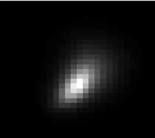
Figure 1:Optical image of geostationary object.
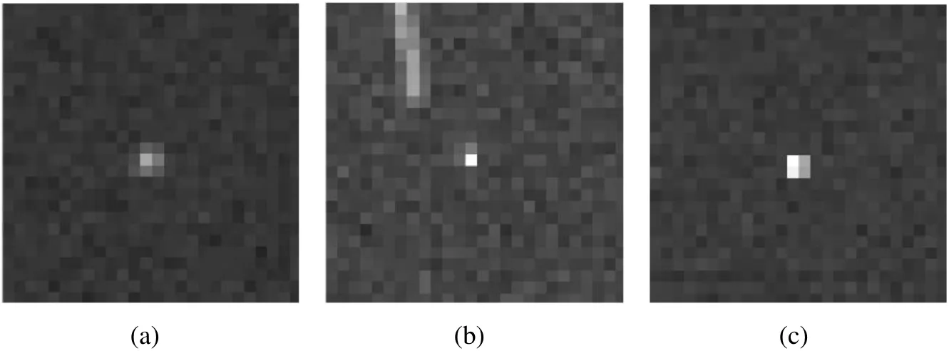
Figure 2:(a)and(b)examples of true object images,(c)example of cosmic ray trace(ZIMLAT,University of Bern AIUB).
Furthermore,not all detections are true detections.Clutter contaminates the measurements.In optical measurements,e.g.cosmic ray events contaminate the measurements;they cannot readily be discriminated from true measurements,as can be seen in Fig.2.Because the objects move relative to the star background and their relative motion is a priori not known,simple stacking techniques to filter out cosmic ray events completely,cannot be used.Alternatively,cosmic filters can be applied to at least reduce the number of clutter measurements[Frueh and Schildknecht(2012)].
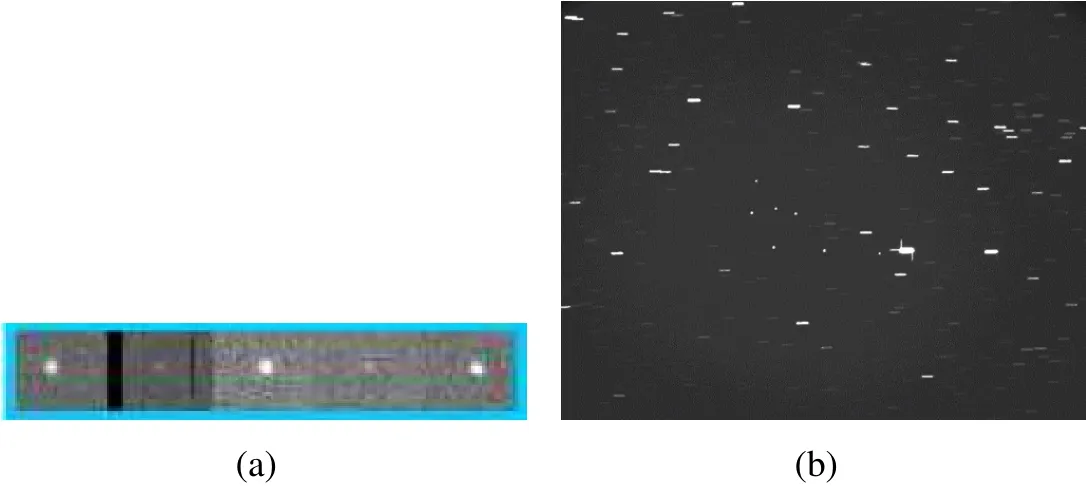
Figure 3:(a)five subsequent images of the same object,spaced by 30 seconds,(b)fi ve geostationary objects in front of star background(ZIMLAT,University of Bern AIUB).
Not every time that the object is actually in the field of view it is also detected.The signal can be below the noise level or e.g.occultation occurs.The attitude motion of objects can be very rapid,leading to large brightness changes in short time intervals;one example of this is shown in Fig.3a.Occultation in optical observations occur when the object is in front of a star,as illustrated in Fig.3b,which shows five geostationary objects in front of the star background[Frueh(2011)].This illustrates how easily occultation can occur in regular observations.
3 PHD filter and Cardinality only PHD filter
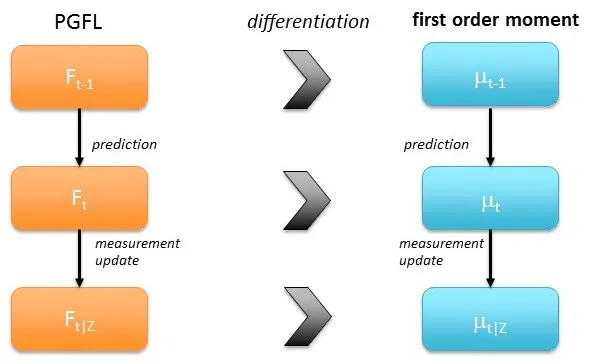
Figure 4:Derivation and data flow steps of the PHD filter.
Instructive derivations of the PHD filter can be found in [Mahler (2007); Houssineau,Delande,and Clark(2013)].Gaussian mixture closed-form PHD filter derivations can be found in Clark,Panta,and Vo(2006);Vo and Ma(2006).Closely following the derivation in[Houssineau,Delande,and Clark(2013)],the formulation of the probability generating functionals(PGFls)Fare used to describe the multi-object population and then differentiated in order to find the first-order moments.
A PGFl is a mapping of an arbitrary functionh:X→[0,1],generated by a series of probabilitiespΦ,associated to a point process Φ:

wherexiare the different realizations of the point process in the spaceX,in our case the state space and the states of the different possible object realizations.A state is defined as position and velocity of the object.E[]is denoting the expectation value.It can easily be seen thatF(0)=pΦ({0}),which is the pdf in the absence of any objects(empty set),andF(1)=1.Fig.4 shows the differentiation and data flow steps of the PHD filter.
For the prediction step,the PGFl has the following form:

whereFt?1(h)is the PGFl describing the population at the previous time step,Fcrea(h)is the PGFl describing the object creation process,psuris the probability of survival,T(xt‖xt?1)is the state transition from the state att?1,denoted as xt?1,to the timet,denoted as xt.x is the set of the individual states of all objects.Eq.2 is derived as the superposition of the surviving objectsFsur(h)and the newly created onesFcrea(h).xt={x1,...,xk}tdescribes the set of the states of the objects at a given time t.It has to be noted that the PGFl is defined on the single object state.
In order to arrive at the final simple form shown in Eq.2,it is assumed that the targets are independent(A1)and that the newborn targets and the surviving ones are independent (A2); the probability of survivalpsuris assumed to be the parameter in a Bernoulli process(A3).A Bernoulli process ? can be defined as follows.For a spatial probability density functionf(x)(Rf(x)dx=1):

for a probability parameterp,which can take values between zero and one.φis the empty set.In the concrete case,this means the target either survives with a probabilitypsur,with a state distributed according tof,or dies with a probability 1?psur.That completely describes the survival-dying process statistically.
The PGFl of the measurement process and the objects can be expressed as:

with the arbitrary functionsh,g:X→[0,1].Gclutis the PGFl of the clutter process,pdis the probability of detection,Lis the likelihood function,and z is the measurement.In the derivation of Eq.5 it is assumed that the measurements are produced independently(A4),the probability of detectionpdcan be modeled a Bernoulli parameter(A5),and that the clutter process producesmeasurementsindependently from the actual objects in the scene(A6).
Utilizing Bayes’rule and the fact that the actual number of measurementsZ=z1,z2,.....,zn(clutter and real object measurements) the sensor has received is known,the PGFl of the data update,derived as the directional derivative of the PGFl in E-q.5,has the following form:

In order to derive the first moments,it is utilized that the first order moment density is the first-order directional derivative of the corresponding PGFl:

This leads to the following filter equations for the first-order moment densities:
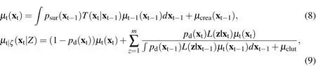
whereμcrearepresents the first moment of the object creation.In order to derive these closed-form expressions,one has to assume that the predicted targets is described by a Poisson point process(A7)and that the point process describing the number of clutter measurements can be modeled as a Poisson process,too(A8).
A simplified form of the PHD filter is the cardinality only version of the PHD filter,which only solves the cardinality problem(not to be confused with the Cardinality PHD filter,CPHD,which also,in addition to the first-order density,propagates the cardinality distribution of the random finite set.The filter equations for the cardinality only PHD filter are the same as in Eq.9,except for the state estimation part.

wheremrepresents the number of measurements.
4 Discussion of the Premises and Assumptions
4.1 Independence of Objects
In the regime of SSA,the assumption(A1)that the objects are independent is most of the time fulfilled.Independence means that the dynamics of the objects are not coupled;that is,one object does not influence the dynamics of the other.The single target differential equation can be written as:
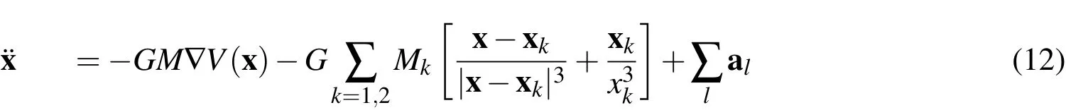
where x is the geocentric position of the object,G the gravitational constant,M the Earth mass and V(x)the Earth gravitational potential,third body gravitational perturbations of the Sun and Moon(k=1,2)with the states xk.Finally,∑a is the sum over all non-gravitational accelerations acting on the satellite.Popular nonconservative perturbations include solar radiation pressure and drag.An object interdependence could only be introduced via those accelerations;realistically,this could be the case for decaying objects and drag wake effects.A further case is on-orbit collisions at time scales where the dynamic effects from the collisions are still dominating.
4.2 Independent Newborn and Surviving Objects
The assumption(A2)that the surviving and newborn objects are independent is an assumption that might be in conflict with the real dynamical situation in the near Earth space.For sure,there is a weak coupling between the surviving targets and new launches,as new launches in part tend to be motivated to refurbish old assets.However,the dead objects still remain in orbit for extended periods of time.More crucial is the object creation that is not caused by new launches but via satellite aging and on-orbit collisions.Following Kessler and Cour-Palais(1978),the collision rate between satellites can be expressed as:

where σ is the spatial density created by the other objects in the volume element dV,ˉv is the average relative velocity,andˉA is the average cross sectional area.Although Kessler’s theory might be controversial in some of his conclusions,the source of debris creation from collisions and impact motivated break-up is valid.Hence,there is a strong and direct coupling between the surviving targets.As with the assumption(A1),a violation can be found in times of tracking through collision events.
4.3 Probability of Survival
Assumption(A3)says that the object either survives with a well-defined probability value,or it dies;probability of survival is represented as the parameter of a(constant)Bernoulli process.Often,in the use of a PHD filter,this quantity is defined as a constant parameter;however,there is no restriction to make it time varying,which is more appropriate for the SSA problem.Object death is only immediately relevant in the strictest sense for objects in decaying orbits;however,sensing limits should not be neglected.In the absence of collisions,the model for the probability of survival can be modeled as the following in the absence of collisions:
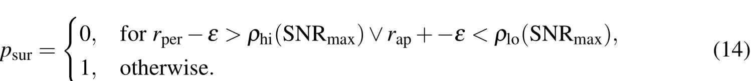
If the perigeerper=(1?e)a(eccentricitye,semi-major axisa)is higher than the upper bound sensing limit,of one or a combined sensor suite,ρhi(SNR(t)),or the apogeerap=(1+e)ais lower than the lower bound sensing limitρlo(SNR(t)),the object has left the sensing scene.No new measurements on the object can safely be expected;it hence is dropped.A precaution against orbital uncertainties can be made with an offsetε.A good choice ofεthen could be defined using the three sigma bound in eccentricity?eand the three sigma bound in semi-major axis?aasε= ?a+2?a·e.The lower sensing limit might coincide with the Earth’s surface.One could imagine the situation in which a target is sought to be keptalivealthough no new measurements can be expected.In that case,a maximum time span since it has left the scene(apogee,perigee condition)can be put as an additional constraint.It has to be noted that the detection limit depends on the signal-to-noise ratio(SNR).In a conservative approach,the maximum signal to noise ratio(SNRmax),in case it is known,should be used,which occurs for minimum phase angle and zenith observations under best conditions.More details on the SNR computation can be found in section 4.5.The probability of survival model as proposed here is hence linked to the probability of detection and can be written as:
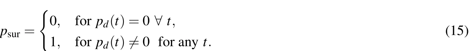
Theoretically,one could also take the specific sensor scheduling scenario into account,which might eliminate further objects;however,it would mean that the sensing schedule can be predicted for all times and excludes detections of objects under potentially growing?aand?e.
The problem of object death in its current form in collisions that destroy the parent object is an instantaneous process that is hard to predict given the state uncertainties in the state propagation.Even when a collision seems certain,it is almost impossible to predict if the parent object remains sufficiently intact to allow for a survival in the classical sense,especially as object sizes and potential overlap in the collision are hardly known.However,as stated above,assumption A1 and A2 would be already violated in the case of a collision.As fatal on-orbit collisions are(fortunately)still very seldom events,with a combined reported and suspected number of five in the past sixty years of space fairing,see Klinkrad,Wegener,Wiedemann,Bendisch,and Krag(2006)and references therein,and best measures are taken to prevent further collisions,probability of survival even when taking collisions into account is still practically one for non-decaying objects within the sensing realm of the sensor suite.This means,even when processes like spawning are integrated in the filter process,it is extremely challenging to incorporate it without a specific trigger or external knowledge,because of the evanescent probability.
4.4 Independence of Measurements
Assumption(A4)requires independence of the measurements.Here,one needs to discriminate between optical measurements and radar measurements.In optical measurements,the measurement is the astrometric position(two angles,such as e.g.right ascension α and declination δ ).A potential coupling of the measurements of different objects that are in the same observation frame is given via the common noise level and the readout process.However,as the background noises are dominated by other celestial sources,such as zodiac light and the background stars and atmospheric scattering,this effect is negligible.Extracting the velocity information from two subsequent frames introduces a huge dependence between the two subsequent measurements:

which is often done for two measurements of the same object that are very close in time together(difference only εt,a small time step relative to the orbital period of the object in question).The dependence can be circumvented in counting the two adjacent measurements only as a single angle and angular rate measurement(α(t1),δ(t1),˙α(t1),˙δ(t1))and not reusing the astrometric position measurement at time t2.Alternatively,angular rates may also be extracted from single exposures.The situation is different for radar measurements.Radar detection methods require coherent pulse to pulse integration,computing the match-function of a set of range and velocity values,see[Markkanen J.(2006);Krag,Klinkrad,Jehn,L.Leushacke,and Markkanen(2007)].Unlike in the optical case,those are normally treated as a single measurement,hence leaving the dependence of the measurements in the data,when they are interpreted the traditional way.
4.5 Probability of Detection
Assumption(A5)states that the probability of detection is modeled as the parameter of a Bernoulli process,hence that the object is either detected with a given probability or not.The probability of detection is directly dependent on the signal to noise ratio(SNR)[Frueh and Jah(2013);Sanson and Frueh(2015,2016)]and time-varying.Albeit it does not contradict the derivation of the PHD filter directly,the probability of detection is often modeled constant,which does not match the SSA situation.Moreover,very low probabilities of detection can occur,which,by construction,the PHD filter has difficulties to deal with.
In order to model the probability of detection correctly,all light that is received at the detector has to be known,and how the detector converts it,and how the signal evaluation process is performed.Albeit,those steps are simple,they are often overlooked.The following discussion can in parts be found in[Sanson and Frueh(2016);Frueh and Jah(2013);Sanson and Frueh(2015)].The signal from the object is dominated by the observation geometry at the time of the observation,the object geometry,and surface properties.In the derivation here,the focus is placed on indirect illumination by the sun;however,the results are easily adapted to active illumination,by shifting the place and strength of the source accordingly.
4.5.1Object Irradiation
The reflected irradiationIat the location of the observer in[W/m2],is:

ISunis the irradiation of the sun at the location of the object for a given wavelengthλ.In general,ISun(ˉλ)·?λmay be approximated with the solar constant,I0=1367.7W/m2;to be more precise,the deviation from the one astronomical unit scaling should be taken into account.ˉλwould be the mean wavelength.The mean should be chosen as the mean of the sensing spectrum of the sensor at hand.Ais the complete area off which the light is reflected,rtopois the topocentric distance(distance object to observer),and Ψ is the phase function.In the approximation,the precise solar spectrum and the spectral response of the object has been neglected and a combined white light response is modeled.For filter measurements,or color CCD sensors,the correct spectral response has to be taken into account.The phase function depends on the object properties,the shape and reflection properties;it defines how the light is reflected off the object for a given incident angle of the light and angle of observation.Ψ can be defined as:
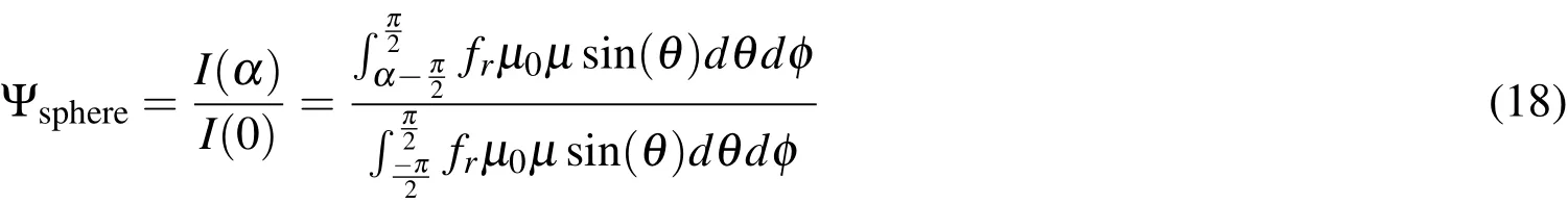
μ0is the incident light direction,μis the outgoing observer direction,andαis the phase angle between the incoming flux and the direction of the observer.In general,the bidirectional reflection model of choice can be applied.In the context of this paper,the surfaces are modeled as a mixture of Lambertian,diffuse reflection and absorption is adapted.For a Lambertian reflectionFor some simple shapes,closed-form solutions for the phase function can be obtained,such as the sphere;without loss of generality,the observer can be placed in the xy plane of the sphere;definingμ0=sinθcosφandμ=sinθcos(φ?α)leads to the well-known result,see Wertz(1978):

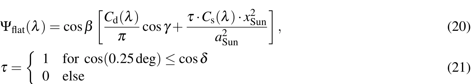
for a diffuse reflection parameterCd(λ).αwould be the classical phase angle(angle between observer,object,sun).In general,real objects are modeled for a mixture between e.g.specular,Lambertian reflection,and absorption.In general,Cd+Cs+Ca=1 for opaque materials.Specular reflection on a sphere is not taken into account here as classical glints cannot be caught from ideally spherical space objects.Glints are only possible from flat surfaces.Spherical surfaces always return light to the observer as long as they are not in the Earth shadow or the illumination source is exactly opposite to the observer.For a flat plate,the integrals over the hemisphere have to be replaced by the integral over the illuminated surface,and are hence very simple.μ0=cosβandμ=cosγfor the flat plate case,whereβis the angle between the direction to the illumination source,S,and the normal vector of the surface,N.γis the angle between the observer O and the normal vector:
4.5.2Celestial Background Irradiation
Besides the irradiation of the object,other background sources also enter the detector.The irradiation of the object is not the only light that is reflected towards the observing sensor.In optical observations,several background sources,such as zodiac light,direct and stray moonlight,atmospheric scattering,and atmospheric glow,may be taken into account.Intensive studies on the background sources and tabulated values can be found in[Daniels(1977)Allen(1973)];application to SSA observations can be found in Frueh and Jah(2013).
For celestial background sources Eq.17 has to be adapted as the following:

Ii(λ)denotes the wavelength dependent exact irradiation values of the different sources.The signal expression in the following equations are derived using the approximation in Eq.22 at the mean optical wavelength of 600nm.
Airglow spectral radiation,IAG(λ),is the faint glow of the atmosphere itself,which is caused by chemiluminescent reactions occurring between 80 and 100 km.The irradiation values can be directly computed from the irradiation valuesJi,as shown in the subsequent equations.Irradiation values are well documented in literature,e.g.in[Daniels(1977)Allen(1973)].Atmospherically scattered light is the sum of all light that is scattered by the atmosphere.Both can be modeled as the following:
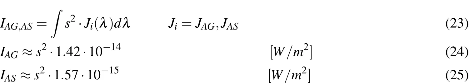
wheresis the angle under consideration,in case of the telescope.It can be chosen to be the field of view(FOV)of the sensor,a field averaged background would then be derived.This is legitimate for small to medium sized FOVs;for wide field telescopes,this approach is not recommended.The most precise modeling is achieved whensis chosen to be the angle that is integrated into a single pixel.
Diffuse galactic light is scattered sunlight by small particles concentrated in the ecliptic.It can be modeled as the following:
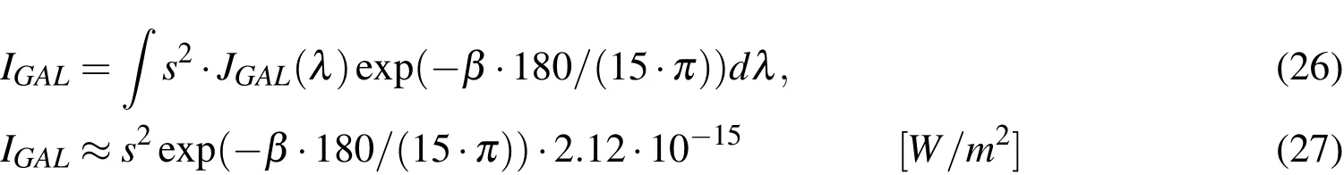
whereJGALis the spectral irradiation at zero galactic latitude(β).Zodiac light is the diffuse stray light from the sun,which is visible in the night sky even long after
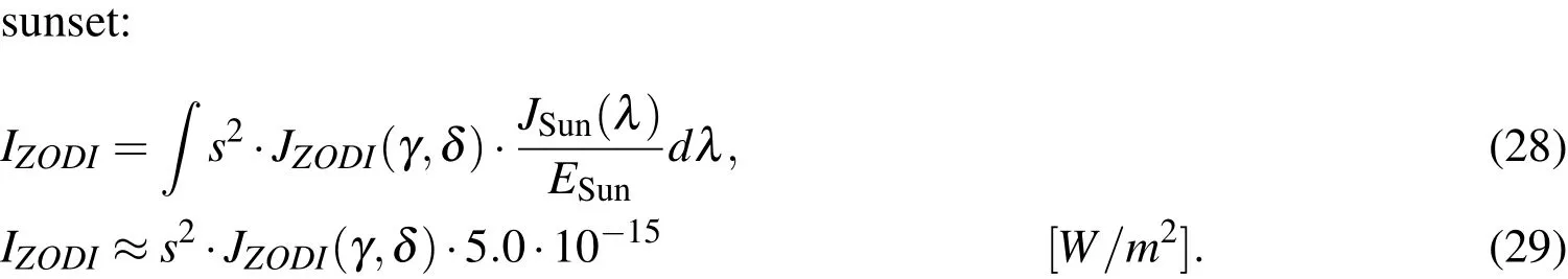
γ,δare the longitude and latitude in ecliptic coordinates andJZODI(γ,δ)is the total irradiation per unit angle.As zodiac light can be by far the strongest background source and has a large variability,the use of the exact tabular values for the total irradiation is recommended.
Another major light source is the faint stars in the background.One way to include stars is to include them at the exact position as they appear in extensive star catalogs.However,this is a very time consuming procedure.Tables exist with the number of stars of given photographic magnitudes,see[Frueh and Jah(2013);Allen(1973)].Using these,they can be converted to radiance values,using the known spectral distribution of faint stars,as in the case of the galaxies.The conversion is done in the blue wavelength(440nm)to have the best equivalence with the photographic magnitudes denoted bym.This leads to the spectral star irradiation:
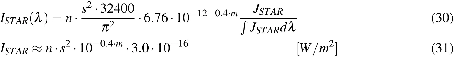
wherenis the number of stars in the assigned bin. The irradiation values correspond to the irradiation without an atmosphere.Sometimes,one is not interested in a specific wavelength,but the total radiation;in this case,one can integrate or use approximations for the white light.
4.5.3 Sensor response
The response to any of the incoming celestial irradiation,from the object of interest or from any of the celestial sources,can be modeled as the following:
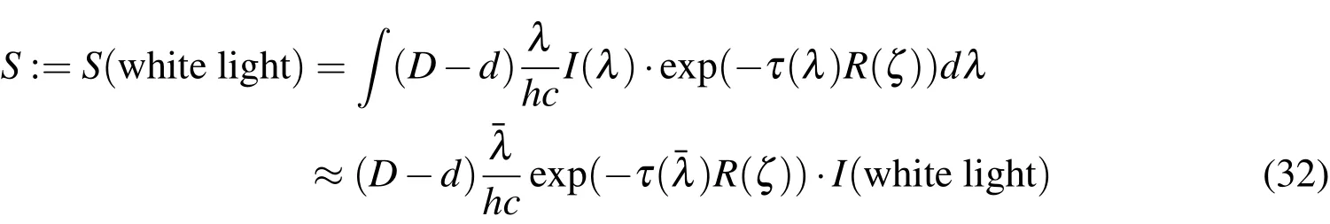
with the speed of light,c,Planck’s constanth,the area of the aperture,D,and the obstruction of the aperture,d.R(ζ)is the van Rhijn factor,which can be approximatedto first order and describes the deviation from the zenith by angleζand the additional air mass and thickness that has to be accounted for in low elevations[Daniels(1977)].A very simple atmospheric extinction model has been adapted,withτbeing the atmospheric extinction coefficient.Note that atmospheric extinction is zero for the airglow and atmospheric scattering signals,because they are created in the atmosphere rather than being extinct via passing through it.
The count rate is derived from the signal via the time integration,dt,during which the sensor is able to catch photons:

whereQis the quantum efficiency.The photon count is a statistical process.A model for the signal and subsequent count at the detector is a Poisson distribution.The approximation neglects the shutter function itself and assumes that the integration time is the same over all the field of view of the sensor.The signal,however,is spread over several pixels,which report their count rates independently.The count rateCis hence interpreted as the mean of a Poisson process.Strictly speaking,quantization already happens at the signal level.However,this is without consequences,as only in the count,the time averaging takes place.The count rates are then transformed via the so-called gain,g,from the count level to the analog to digital units(ADU)that are read out electronically.The gain is not completely linear over all counts of the sensor,although a linearity of the gain is desired.Non-linearity normally occurs when reaching the saturation level of the sensor.In the process of the transformation,a truncation takes place as normally only integer ADU values can be reported.
For simplicity,it is assumed that the complete irradiation is counted in a single pixel.Depending on the pixel size in combination with the setup of the optics,the Airy disk diffraction pattern that is formed is counted in several adjacent pixels.In this case,normally only the pixel counts of the first maximum are taken into account,which is around 84%of the total count of the complete diffraction pattern.This is especially true if the object is moving relative to the sensor.
The sensor itself introduces additional counts,so-called dark noise,that stem from electron fluctuations that occur even when the shutter remains closed.The readout process itself creates readout noise.
4.5.4Probability of Detection
The probability of detectionPDcan be defined as the following(for further details,please also see Sanson and Frueh(2015,2016)):

where SOBJis the object signal,modeled as the mean of a Poisson distribution,and N is the cumulative noise.Again,it is assumed that the signal is integrated in a single pixel.Following the derivation of[Merline and Howell(1995)],the noise can be represented as:
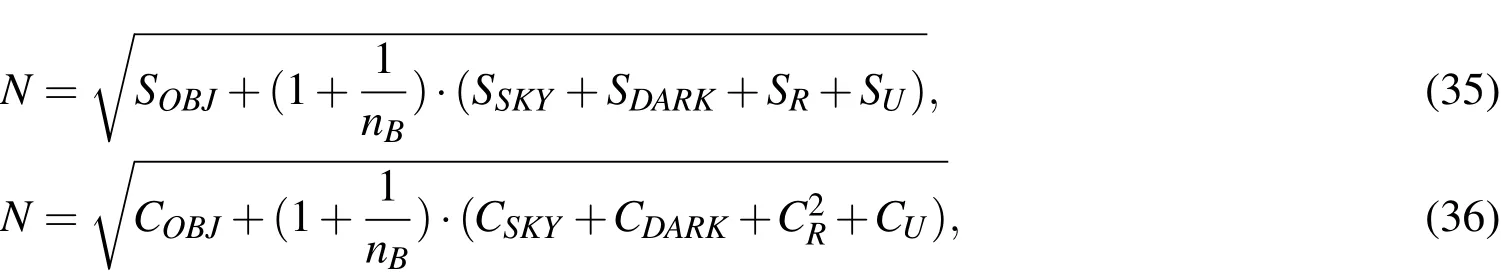
where SSKYis the variance of the celestial background sources,modeled as a Poisson distribution with the count rate as the parameterCSKY.SDARKis the mean of the dark noise,modeled as a Poisson distribution with the parameter CDARK,is the readout noise,which by the central limit theorem is modeled as Gaussian distributed with the variance of a Gaussian distribution,and SUis the truncation noise variance,which approximately can be modeled as uniformly distributed,rendering the variance CU=g2/12,where g is the gain.nBis the number of pixels that have been used in the background determination.For the derivation of the CCD equation,including improved modeling for cases,when the source is not integrated in a single pixel,see Sanson and Frueh(2015,2016).Inserting it into the probability of detection formula:
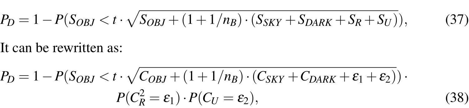
which allows to evaluate the different distributions in a cumulative density function for the Poisson distributed parts and conditional probability density function on the remaining terms:

4.6 Clutter
Assumptions(A6)and(A8)focus on the clutter process.The assumption that clutter and measurements are produced independently is easily fulfilled,as the physical processes that are generating the object signal and the clutter signal,such as the cosmic ray events in the optical observation,are independent.The signal of the object is the irradiation from the object,either stemming from the sun or from the observation station and is radiated back to the observer.Clutter,such as cosmic ray events,are charged particles that accidentally impinge on the sensor.No part of the measurement process excites or influences the charged particles that arrive at the detector.Cosmic ray events are a textbook example of a Poisson process that describes the arrival of the charged particles at no distinct order at this time integrated process.
4.7 Predicted Object Distribution
Assumption(A7),that the predicted object distribution is a Poisson process,is one of the most crucial ones.As we have seen in Eq.12,the underlying dynamics is of course purely deterministic,even though sometimes,exact knowledge on all parameters is missing.Together with the way objects are created or die,single outbursts in the population in crucial collisions,and a few launches and decays,the object population cannot readily be suspected to be in a close resemblance of a Poisson process.In the previous section,no weighting is applied in the filter equations,which means the filter is highly responsive at each new time step.A Poisson process implies that the actual number of targets can jump,same as it accurately applies to the clutter population that is detected.Actual jumps in the factual populations only happen in collisions,which are rare and problematic as discussed above already.The actual population is concentrated in certain orbits and not highly variable,hence the predicted object population on the observation frames is highly dependent on the specific observation scenario.In actively tracking specific objects,often called follow-up tracking,in contrast to so-called blind tracking or surveying,it is expected that the objects that are visible in the observation frames is more or less constant.
It can be seen that the filter is put to its edges already with the birth and death processes,which takes on extreme values and does not settle on the middle ground.This is in connection to the Poisson process assumption for the object population,which might be highly inadequate.
5 Simulation Results
Simple tests to show the impact of the modeling parameters on the filter performance have been run.Five different variations of the same scenario have been created.For the tests,the cardinality only version of the PHD filter has been used,hence only the number of targets is estimated.In the filter there is hence no explicit state dependence.As explained above,this makes the analysis independent of specific solutions for problems of first orbit determination and propagation.However,it already illustrates the general filter performance under model mismatch.In order to adequately supply the Cardinality only filter,all state dependent values are assumed to be identical for each target.
The scenario is chosen as the optical observation of the ASTRA satellite cluster.The ASTRA cluster is located in the geostationary ring.It is assumed that the telescope is in staring mode and the objects are in the field of view at all times,displayed in Fig.3b.The scenario comprises of 100 seconds and measurements every 10 seconds.The phase angle can be assumed to be nearly constant during such a small time period,the solar panels are roughly aligned with the sun direction,and a three degree offset is assumed.The direction to the observer is 80 degrees.The angles are assumed fixed in the filter.Motion of the sun and the observer are negligible in the 100 second scenario.ASTRA satellites are at a distance of 36,000 km.The solar panel area(which dominates the reflection)can be assumed to be around 45 square meters(based of the dimensions of retired ASTRA 1B).Solar panels have an absorption coefficient of around 0.3,a specular component of around 0.5,and a diffuse component of 0.2.Under these observation conditions,the ASTRA satellites have a magnitude of 12.ASTRA satellites are large space objects and they appear very bright on the night sky under small observation angles.The current large observation angle is chosen to illustrate the effect of different sensors even on relatively large,stabilized(constant angle to the sun)objects.In the simulations,a gain of 0.1 is assumed,a readout noise of 100 ADU,a sky background of 5,000,000 ADU,and an exposure time of 1 second is modeled;for the background estimation,it is assumed the whole detector of 2000 by 2000 pixels have been used.Each scenario is run 1000 times.In order to measure and illustrate the performance,the average of all runs is plotted,and the mean sample error can be evaluated:

where m(t)is the true number of objects,five in the chosen scenarios,?m(t)is the estimated number of targets,and the number of runs in the simulation,n,is 1000.It has to be noted that within the filter,non-integer values for the number of objects are allowed.Accordingly,the sample variance is computed:

Scenario 1 is the baseline scenario.No clutter is assumed,the number of true objects stays constant combined with a high probability of detection of 1.0,which corresponds to a large aperture telescope observation of one meter.In the second scenario,realistic large aperture observations are assumed with a high quality camera,which means that clutter is also present.In the third scenario,a small aperture is assumed and camera performance parameters are slightly decreased, where either of those factors decreases the probability of detection.Clutter is also present.In scenarios 4 and 5,variable probability of detection is modeled,which corresponds to the ASTRA satellites after attitude control has been disabled.Natural torques lead to attitude motion,which is reflected in a varying signal to noise ratio and,ultimately,in a non-static probability of detection.A mid-sized aperture is assumed.In scenario 4,the filter models the change in the probability of detection exactly according to the truth model,in scenario 5,the filter assumes a constant probability of detection,whereas the true probability of detections is time-varying,same as in scenario 4.
5.1 Scenario 1
Scenario one is a baseline scenario;a one meter aperture telescope is assumed with 10 cm obstruction and a very high quantum efficiency of 0.97.The probability of detection is 1.0,despite the large observation angle,and the signal to noise ratio at the detector is 23.2.A detection threshold of t=2.5 is assumed.The five objects in the cluster are in the field of view during the whole scenario,and no objects are created nor lost.Object birth is assumed to be practically zero(10?15),and probability of survival is 1.0.It is assumed that no clutter would be present and that the filter is initialized with the correct number of objects(5),both unrealistic assumptions.Apart from the fixed number of objects,all assumptions of the filter are met.Not surprisingly,the filter performance is also perfect;at every time of the scenario,the correct cardinality is estimated,also illustrated in 5.
5.2 Scenario 2
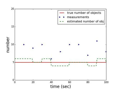
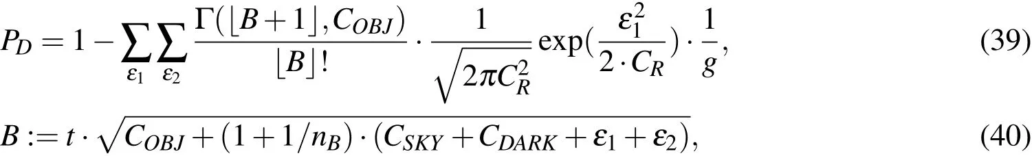
Figure 6:Scenario 2,one arbitrary solution in the Monte Carlo trials:True number of objects(red),the cardinality of the measurements(true measurements plus clutter every ten seconds(blue))and the filter estimate(dashed green).
In the second scenario,clutter was added.The clutter is modeled to be Poisson distributed with a parameter of 4.Probability of detection is still 1.0.The remaining parameters are modeled like in scenario 1.This would correspond to observations with a large one meter aperture telescope and 10 centimeter obstruction,with a realistic clutter process caused by cosmic ray events.The actual number of cosmic ray events varies by location and sensor specifics,as some sensor materials themselves are very radioactive on a low level.A Monte Carlo simulation of 1000 trials has been conducted.Fig.6 shows one trial scenario outcome from the Monte Carlo simulations,where the estimated number of objects are rounded to the closest integer in the display(inside the filter,floating point numbers of the estimated number of objects for the computation are kept).It shows that in the mismatch of the object population distribution,despite the high and correctly modeled probability of detection of 1.0,the filter does not match the true object population.Fig.7 shows the average over all trials without rounding.The error,standard deviation,and the deviation from the true number of observations.As the probability of detection is one,the number of observations is overshooting.Not surprisingly,the average number of observations above the correct number of objects is very close to the Poisson parameter of 4.The error in the number of objects that are estimated is not stable.The one sigma standard deviation does not envelope the true averaged error that is found in the simulations.The error in the estimate reaches around six percent maximally in the scenario.
Figure 7:Scenario 2:(a)sample mean error(red),one standard deviation(green);(b)difference in the average number of measurements and the true object number.
5.3 Scenario 3
In scenario three,it is assumed that a smaller aperture telescope of 10 centimeter is used.The obstruction is 0.5 centimeters.The camera is assumed to have a quantum efficiency of 0.8.The signal to noise ratio in this case would be 2.2.A detection threshold of t=2.5 is assumed.This leads to a probability of detection of around 0.3.Fig.8 shows one sample trial of the Monte Carlo simulation.Because of the low probability of detection,the number of objects is consistently underestimated.
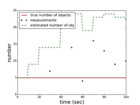
Figure 8:Scenario 3,one arbitrary solution in the Monte Carlo trials:True number of objects(red),the cardinality of the measurements(true measurements plus clutter every ten seconds(blue))and the filter estimate(dashed green).
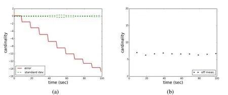
Figure 9:Scenario 3:(a)sample mean error(red),one standard deviation(green);(b)difference in the average number of measurements and the true object number.
Fig.9a shows the error and standard deviation,and Fig.9b shows the difference in the number of measurements and the true number of objects that are in the field of view.Because of the low probability of detection,on average,six to seven observations are made(true objects and clutter)with a clutter Poisson distribution with parameter four.The error statistic shows that the estimate is consistently off and seems to worsen the longer the scenario lasts.The error is significantly larger as in the previous case and builds up to over 300 percent.The model mismatch consists of the static object numbers and the assumption of a Poisson process in the predicted number of objects.The filter is stressed by the very low probability of detection in the presence of significant clutter.However,the scenario is not unrealistic.Low probabilities of detection can,as outlined above,even occur for large objects,under large observation or phase angles,even when the objects are stabilized and the angle to the sun is optimal.Small apertures lead to lower probability of detections in optical sensors than larger apertures for the same observation conditions.The performance of the sensor also has an influence,albeit to a lesser degree.The ASTRA satellites are among the largest objects in the geostationary ring,and the area of the solar panels is tremendous.Any smaller object with comparable reflection values,or less reflective objects of the same size,will have a lower signal to noise ratio,which in turn then can lead to a low probability of detection.Exceptions are glint conditions.
5.4 Scenario 4
In the fourth scenario,a mid-sized aperture is assumed of 50 centimeters and a 3 centimeter obstruction.Instead of assuming stabilized satellites that have a constant angle towards the sun and a slowly changing angle towards the observer,it is assumed that the satellites slowly rotate around the axis perpendicular to the solar panels.In the absence of stable active attitude control,natural torques induce rotation.The situation is also comparable to spin stabilized satellites with a very heterogeneous outer surfaces.The satellite solar panels are assumed to move from an angle of 35 degrees to the observer and 25 degrees to the sun,continuously to 85 degrees to the observer and 75 degrees to the sun,respectively.With a quantum efficiency of the camera of 0.9,this leads to a change in the signal to noise ratios of 97 to 3.The probability of detection accordingly changes from initially 1.0 for seven of the ten measurements and then reaches values of 0.99,0.87,and 0.23.A detection threshold of 2.5 is assumed again.In the filter,the truth of the probability of detection is exactly matched.Fig.10 shows a sample trial of the scenario.It can be seen that the filter changes from underestimating to overestimating the number of objects when the probability of detection changes from values of one in the first measurements to lower values,although the filter is updated with the correct values for the probability of detection.Fig.11 shows the that consistently the error is increasing as the probability of detections are lowered values towards the end of the scenario.The number of measurements on average is stable around four,the Poisson parameter of the clutter process,and then drops as not all objects are detected any more.Overall,the performance of the filter is better than with consistently low probability of detection values.The error reaches only around 7 percent.
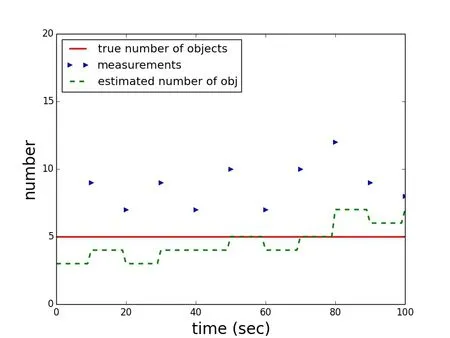
Figure 10:Scenario 4,one arbitrary solution in the Monte Carlo trials:True number of objects(red),the cardinality of the measurements(true measurements plus clutter every ten seconds(blue))and the filter estimate(dashed green).
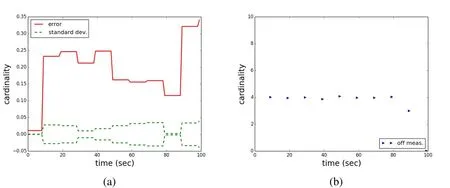
Figure 11:Scenario 4:(a)sample mean error(red),one standard deviation(green);(b)difference in the average number of measurements and the true object number.
5.5 Scenario 5
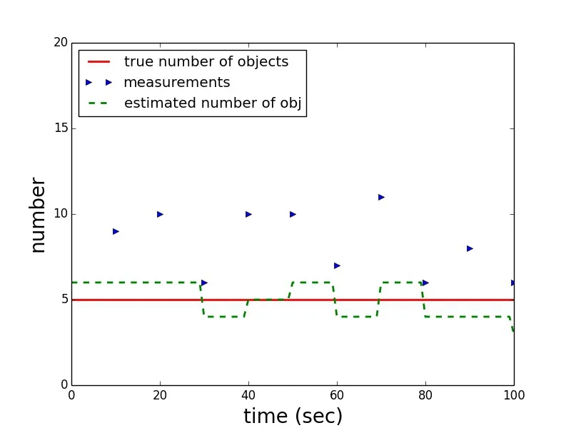
Figure 12:Scenario 5,one arbitrary solution in the Monte Carlo trials:True number of objects(red),the cardinality of the measurements(true measurements plus clutter every ten seconds(blue))and the filter estimate(dashed green).
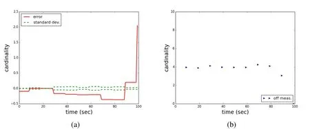
Figure 13:Scenario 5:(a)sample mean error(red),one standard deviation(green);(b)difference in the average number of measurements and the true object number.
Scenario five is a replica of scenario four,except that the filter is provided with a constant value of the probability of detection of the correct but constant average value for the scenario of 0.91.For the generation of the measurements,the correct probability of detection sequence of 1.0 for seven of the ten measurements and the values of 0.99,0.87,and 0.23 for the remaining three measurement times,respectively,is used. Fig.12 shows one trial of the Monte Carlo simulations.It can be seen that in this case the number of objects is constantly either over or under-estimated and that the estimation error increases in the last observation,where the true probability of detection and the averaged one used in the filter differ the most.This trend that is visible in the single trial is supported by the complete Monte Carlo simulation.The mean sample error is larger throughout the scenario compared(be aware of the different scales)to the same scenario with the correctly modeled probability of detection(scenario 4).Although the performance is still in the same order of magnitude at the beginning of the scenario when the large probability of detections are dominated,towards the end of the scenario,when the small probability of detections are reached,the error dramatically increases and reaches values of 40 percent.It appears that the filter is performing comparably with the averaged to the true probability of detection as long as truth and average are both high and relatively close to one another.The filter performance worsens when truth and average probability of detection differ significantly.
6 Conclusions
Finite set statistics based filters have advantages because they offer a fully probabilistic description of a tracking scenario.First order approximations,such as in the cardinality only PHD,have become increasingly popular.In this paper,the filter assumptions that are made in the PHD filter derivation have been compared to the reality of space situational awareness(SSA)tracking.It has been found that,especially in dedicated tracking,a potential mismatch between the predicted object distribution might exist.Probability of survival and object birth are put to their extreme in SSA,especially in the absence of collisions.Collisions pose specific challenges,such as,among others,a model mismatch in target independence.Measurement independence assumptions require careful measurement treatment and potential redefinition especially in radar measurements.A special focus has been laid on the correct definition of the probability of detection.Scenarios have been run,mimicking a simple SSA tracking of five objects of the ASTRA cluster in the geostationary ring.For the simulations,the cardinality only part of the PHD filter has been utilized.Although state dependence has been lost,it provides the advantage to investigate crucial parts of the full PHD filter performance without committing to and independent of a specific method for object propagation and initial orbit determination.
The simulations suggest that,in the presence of realistic clutter,the mean sample error is of the order of ten percent,even when the probability of detection is one,and object birth and death are perfectly known and the predicted object population is the only potential model mismatch.Performance significantly worsens with low probability of detection,leading to mean sample errors of several hundred percent,even when perfectly matched in the filter.Using a time varying probability of de-tection leads to consistent results with the constant probability of detection.Results are significantly worsened when an average probability of detection is used,especially when the average and the true probability of detection differ significantly.In all cases,the standard variation was small relative to the mean sample error.
Acknowledgement:I would like to acknowledge the fruitful collaboration with Prof.Dr.Daniel Clark and his research group,in particular Dr.Emmanuel Delande,from Heriot Watt University,Edinburgh,UK.I am very thankful for all the useful discussions.The work was supported by the VIBOT summer scholar program.
Allen,C.(1973):Astrophysical Quantities.The Athlone Press,University of London,London.ISBN:0 485 11150 0.
Bar-Shalom,Y.(1978): Tracking methods in a multitarget environment.Automatic Control,IEEE Transactions on,vol.23,no.4,pp.618–626.
Blackman,S.S.;Popoli,R.(1999):Design and analysis of modern tracking systems.Artech House.
Blair,W.D.;Bar-Shalom,Y.(Eds):Multitarget-Multisensor Tracking:Applications and Advances(Volume III).Artech House.
Cheng,Y.;DeMars,K.J.;Frueh,C.;Jah,M.K.(2013):Gaussian mixture phdfilter for space object tracking.No.AAS 13-242 in Advances in the Astronautical Sciences.
Cheng,Y.;Frueh,C.;DeMars,K.J.(2013):Comparisons of phd filter and cphdfilter for space object tracking.No.AAS 13-770 in Advances in the Astronautical Sciences.
Clark,D.E.;Panta,K.;Vo,B.-N.(2006):The GM-PHD Filter Multiple Target Tracker.InInformation Fusion,Proceedings of the 9th International Conference on,pp.1–8.
Daniels,G.(1977): A Night Sky Model for Satellite Search Systems.Optical Engineering No 1,vol.16,pp.66–71.
DeMars,K.J.;Hussein,I.I.;Frueh,C.;Jah,M.K.;Erwin,R.S.(2015):Multiple-object space surveillance tracking using finite-set statistics.Journal of Guidance,Control,and Dynamics.doi:10.2514/1.G000987.
Flohrer,T.;Schildknecht,T.;R.St?veken,E.(2005):Performance Estimation for GEO Space Surveillance.Advances in Space Research,vol.35,no.7,pp.1226–1235.
Frueh,C.(2011):Identification of Space Debris.Shaker Verlag,Aachen.ISBN:978-3-8440-0516-5.
Frueh,C.;Jah,M.(2013):Detection Probability of Earth Orbiting Using Optical Sensors.InProceedings of the AAS/AIAA Astrodynamics Specialist Conference,Hilton Head,SC.13-701.
Frueh,C.;Schildknecht,T.(2012): Object Image Linking of Objects in Near Earth Orbits in the Presence of Cosmics.Advances in Space Research,vol.49,pp.594–602.
Gehly,S.;Jones,B.;Axelrad,P.(2014):An AEGIS-CPHD Filter to Maintain Custody of GEO Space Objects with Limited Tracking Data.InAdvanced Maui Optical and Space Surveillance Technologies Conference,pg.25.
Houssineau,J.;Delande,E.;Clark,D.E.(2013):Notes of the Summer School on Finite Set Statistics.Technical report,2013.arXiv:1308.2586.
Jia,B.;Pham,K.;Blasch,E.;Shen,D.;Wang,Z.;Chen,G.(2014): Cooperative space object tracking using consensus-based filters.InInformation Fusion(FUSION),2014 17th International Conference on,pp.1–8.
Jones,B.;Vo,B.-N.(2015):A Labelled Multi-Bernoulli Filter for Space Object Tracking.InProceedings of the 23rd AAS/AIAA Spaceflight Mechanics Meeting,Williamsburg,VA,January 11-15.
Kelecy,T.;Jah,M.;DeMars,K.(2012): Application of a multiple hypothesisfilter to near GEO high area-to-mass ratio space objects state estimation.Acta Astronautica,vol.81,pp.435–444.
Kessler,D.;Cour-Palais,B.(1978): The creation of a debris belt.Journal of Geophysical Research,vol.83,no.A6,pp.2637–2646.
Klinkrad,H.;Sdunnus,H.(1997):Concepts and applications of the{MASTER}space debris environment model.Advances in Space Research,vol.19,no.2,pp.277–280.
Klinkrad,H.;Wegener,P.;Wiedemann,C.;Bendisch,J.;Krag,H.(2006):Space Debris:Models and Risk Analysis,chapter Modeling of the Current Space Debris Environment.Springer Berlin Heidelberg,2006.
Krag,H.;Klinkrad,H.;Jehn,R.;L.Leushacke;Markkanen,J.(2007):Detection of small-size space debris with the fgan and eiscat radars.In7th Workshop,Naval Postgraduate School Monterey,California.
Kreucher,C.M.;Kastella,K.D.;Hero III,A.O.(2004): Tracking Multiple Targets Using a Particle Filter Representation of the Joint Multitarget Probability Density.InSignal and Data Processing of Small Targets,Proceedings of SPIE,volume 5204,pp.258–269.
Merline,W.;Howell,S.(1995): A realistic model for point-sources imaged on array detectors:The model and initial results.Experimental Astronomy,vol.6,pp.163–210.
Mahler,R.P.S.(2007):Statistical Multisource-Multitarget Information Fusion.Artech House.
Markkanen J.,Postila M.,v.E.A.(2006):Small-size Space Debris Data Collection with EISCAT Radar Facilities.Technical report,2006.Final Report of ESOC Contract No.18575-/04/D/HK(SC).
Musci,R.(2006):Identification and Recovery of Objects in GEO and GTO to Maintain a Catalogue of Orbits.Astronomical Institute,University of Bern.PhD thesis.
Musci,R.;Schildknecht,T.;Ploner,M.(2004): Orbit Improvement for GEO Objects Using Follow-up Obervations.Advances in Space Research,vol.34,no.5,pp.912–916.
Musci,R.;Schildknecht,T.;Ploner,M.;Beutler,G.(2005):Orbit Improvement for GTO Objects Using Follow-up Obervations.Advances in Space Research,vol.35,no.7,pp.1236–1242.
Oswald,M.;Krag,H.;Wegener,P.;Bischof,B.(2004): Concept for an Orbital Telescope Observing the Debris Environment in GEO.Advances in Space Research,vol.34,no.5,pp.1155–1159.
Potter,A.(1995): Ground-Based Optical Observations of Orbital Debris:A Review.Advances in Space Research,vol.16,no.11,pp.(11)35–(11)45.
Reid,D.(1979):An Algorithm for Tracking Multiple Targets.Automatic Control,IEEE Transactions on,vol.24,no.6,pp.843–854.
Sanson,F.;Frueh,C.(2015): Noise Quantification in Optical Observations of Resident Space Objects for Probability of Detection and Likelihood.InAAS/AIAA Astrodynamic Specialist Conference,Vail,CO.15-634.
Sanson,F.;Frueh,C.(2016): Probability of Detection and Likelihood:Application to Optical Unresolved Space Object Observation.Celestial Mechanics and Dynamical Astronomy.
Singh,N.;Poore,A.;Sheaff,C.;Aristoff,J.;Jah,M.(2013):Multiple Hypothesis Tracking(MHT)for Space Surveillance:Results and Simulation Studies.InAdvanced Maui Optical and Space Surveillance Technologies Conference,pg.16.
US Air Force(2016):Celestrack Database based on two line elements,supported by CSSI.http://celestrak.com,2016a.
US Air Force(2016): United States Strategic Command Website.http://www.stratcom.mil/factsheets/jspoc/,2016b.
Vo,B.-N.;Ma,W.-K.(2006):The gaussian mixture probability hypothesis density filter.Signal Processing,IEEE Transactions on,vol.54,no.11,pp.4091–4104.
Wertz,J.(1978):Spacecraft Attitude Determination and Control.Volume 73.D.Reidel Publishing Company,Dordrecht:Holland.ISBN:90-277-0959-9.
1Purdue University,West-Lafayette,IN,USA.