Residual-driven Fuzzy C-Means Clustering for Image Segmentation

Cong Wang, Witold Pedrycz, Fellow, IEEE, ZhiWu Li, Fellow, IEEE, and MengChu Zhou, Fellow, IEEE

Abstract—In this paper, we elaborate on residual-driven Fuzzy C-Means (FCM) for image segmentation, which is the first approach that realizes accurate residual (noise/outliers) estimation and enables noise-free image to participate in clustering. We propose a residual-driven FCM framework by integrating into FCM a residual-related regularization term derived from the distribution characteristic of different types of noise. Built on this framework, a weighted ?2-norm regularization term is presented by weighting mixed noise distribution, thus resulting in a universal residual-driven FCM algorithm in presence of mixed or unknown noise. Besides, with the constraint of spatial information, the residual estimation becomes more reliable than that only considering an observed image itself. Supporting experiments on synthetic, medical, and real-world images are conducted. The results demonstrate the superior effectiveness and efficiency of the proposed algorithm over its peers.

I. INTRODUCTION

AS an important approach to data analysis and processing,

fuzzy clustering has been widely applied to a number of visible domains such as pattern recognition [1], [2], data mining [3], granular computing [4], and image processing [5].One of the most popular fuzzy clustering methods is a Fuzzy C-Means (FCM) algorithm [6]–[8]. It plays a significant role in image segmentation; yet it only works well for noise-free images. In real-world applications, images are often contaminated by different types of noise, especially mixed or unknown noise, produced in the process of image acquisition and transmission. Therefore, to make FCM robust to noise,FCM is refined resulting in many modified versions in two main ways: 1) introducing spatial information into its objective function [9]–[14] and 2) substituting its Euclidean distance with a kernel distance (function) [15]–[22]. Even though such versions improve its robustness to some extent,they often fail to account for high computing overhead of clustering. To balance the effectiveness and efficiency of clustering, researchers have recently attempted to develop FCM with the aid of mathematical technologies such as Kullback-Leibler divergence [23], [24], sparse regularization[25], [26], morphological reconstruction [24], [27]–[29] and gray level histograms [30], [31], as well as pre-processing and post-processing steps like image pixel filtering [32],membership filtering [30] and label filtering [26], [32], [33].To sum up, the existing studies make evident efforts to improve its robustness mainly by means of noise removal in each iteration or before and after clustering. However, they fail to take accurate noise estimation into account and apply it to improve FCM.

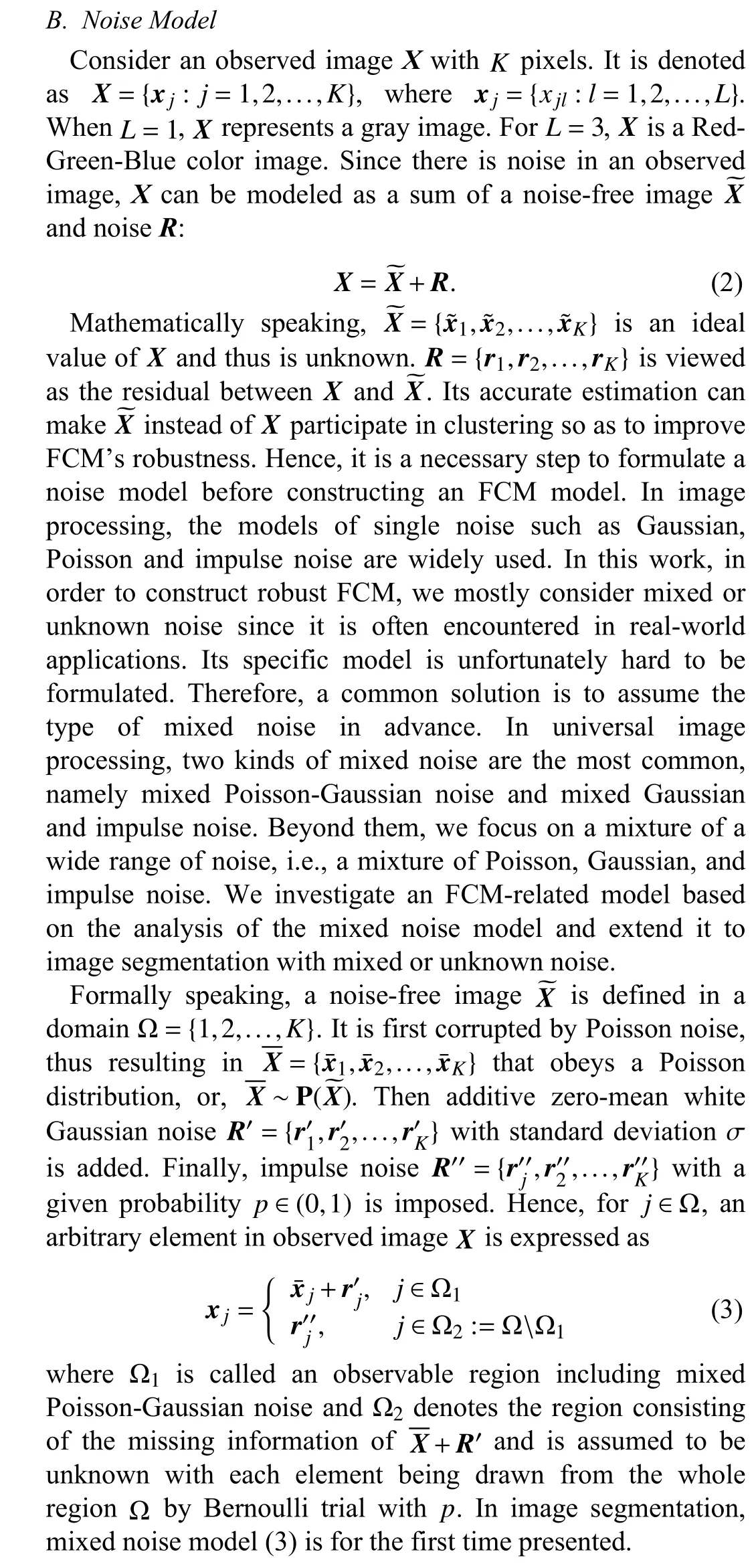
Generally speaking, noise can be modeled as the residual between an observed image and its ideal value (noise-free image). Clearly, its accurate estimation is beneficial for image segmentation as noise-free image instead of observed one can then be used in clustering. Most of FCM-related algorithms suppress the impact of such residual on FCM by virtue of spatial information. So far, there are no studies focusing on developing FCM variants based on an in-depth analysis and accurate estimation of the residual. To the best of our knowledge, there is only one attempt [34] to improve FCM by revealing the sparsity of the residual. To be specific, since a large proportion of image pixels have small or zero noise/outliers, ?1-norm regularization can be used to characterize the sparsity of the residual, thus forming deviation-sparse FCM (DSFCM). When spatial information is used, it upgrades to its augmented version, named as DSFCM_N. Their residual estimation is realized by using a soft thresholding operation. In essence, such estimation is only applicable to impulse noise having sparsity. Therefore, neither of them can achieve highly accurate residual estimation in the presence of different noise.

Motivated by [34], to address a wide range of noise types,we elaborate on residual-driven FCM (RFCM) for image segmentation, which furthers FCM’s performance. We first design an RFCM framework, as shown in Fig.1(b), by introducing a regularization term on residual as a part of the objective function of FCM. This term makes residual accurately estimated. It is determined by a noise distribution,e.g., an ?2-norm regularization term corresponds to Gaussian noise and an ?1-norm one suits impulse noise.

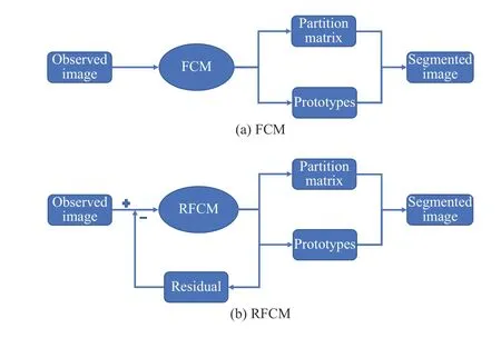
Fig.1. A comparison between the frameworks of FCM and RFCM. (a)FCM; and (b) RFCM.

In real-world applications, since images are often corrupted by mixed or unknown noise, a specific noise distribution is difficult to be obtained. To deal with this issue, by analyzing the distribution of a wide range of mixed noise, especially a mixture of Poisson, Gaussian and impulse noise, we present a weighted ?2-norm regularization term in which each residual is assigned a weight, thus resulting in an augmented version namely WRFCM for image segmentation with mixed or unknown noise. To obtain better noise suppression, we also consider spatial information of image pixels in WRFCM since it is naturally encountered in image segmentation. In addition,we design a two-step iterative algorithm to minimize the objective function of WRFCM. The first step is to employ the Lagrangian multiplier method to optimize the partition matrix,prototypes and residual when fixing the assigned weights. The second step is to update the weights by using the calculated residual. Finally, based on the optimal partition matrix and prototypes, a segmented image is obtained.

This study makes fourfold contributions to advance FCM for image segmentation:

1) For the first time, we propose an RFCM framework for image segmentation by introducing a regularization term derived from a noise distribution into FCM. It relies on accurate residual estimation to greatly improve FCM’s performance, which is absent from existing FCMs.

2) Built on the RFCM framework, WRFCM is presented by weighting mixed noise distribution and incorporating spatial information. The use of spatial information makes resulting residual estimation more reliable. It is thus regarded as a universal RFCM algorithm for coping with mixed or unknown noise.

3) We design a two-step iterative algorithm to realize WRFCM. Since only ?2vector norm is involved, it is fast by virtue of a Lagrangian multiplier method.

4) WRFCM is validated to produce state-of-the-art performance on synthetic, medical and real-world images from four benchmark databases.

The originality of this work comes with a realization of accurate residual estimation from observed images, which benefits FCM’s performance enhancement. It achieves more accurate residual estimation than DSFCM and DSFCM_N introduced [34] since it is modeled by an analysis of noise distribution characteristic replacing noise sparsity. In essence,the proposed algorithm is an unsupervised method. Compared with commonly used supervised methods such as convolutional neural networks (CNNs) [35]–[39] and dictionary learning [40], [41], it realizes the residual estimation precisely by virtue of a regularization term rather than using any image samples to train a residual estimation model. Hence, it needs low computing overhead and can be experimentally executed by using a low-end CPU rather than a high-end GPU, which means that its practicality is high. In addition, it is free of the aid of mathematical techniques and achieves the superior performance over some recently proposed comprehensive FCMs. Therefore, we conclude that WRFCM is a fast and robust FCM algorithm. Finally, its minimization problem involves an ?2vector norm only. Thus it can be easily solved by using a well-known Lagrangian multiplier method.

Section II details the conventional FCM and the proposed methodology. Section III reports experimental results.Conclusions and some open issues are given in Section IV.

II. FCM AND PROPOSED METHODOLOGY

A. Fuzzy C-Means (FCM)

Given is a set X={xj∈RL: j=1,2,...,K}, where xjcontains L variables, i.e., xj=(xj1,xj2,...,xjL)Twith T being the transpose of a vector. FCM is applied to cluster X by minimizing:

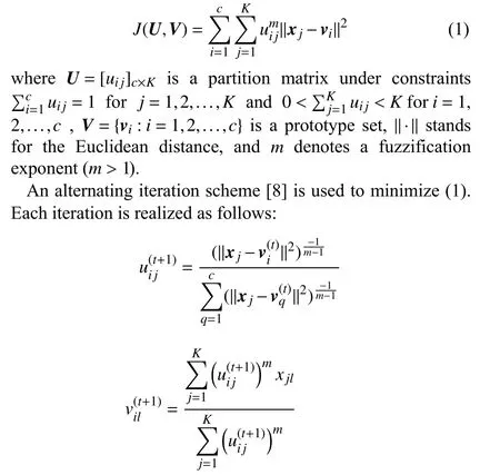
where t=0,1,2,..., is an iterative step and l=1,2,...,and L.By presetting a threshold ε, the procedure stops when ‖U(t+1)?U(t)‖<ε.

C. Residual-driven FCM

Since there exists an unknown noise intensity in an observed image, the segmentation accuracy of FCM is greatly impacted without properly handling it. It is natural to understand that taking a noise-free image (the ideal value of an observed image) as data to be clustered can achieve better segmentation effects. In other words, if noise (residual) can be accurately estimated, the segmentation effects of FCM should be greatly improved. To do so, we introduce a regularization term on residual into the objective function of FCM.Consequently, an RFCM framework is first presented

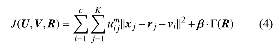
where β={βl:l=1,2,...,L} is a parameter set, which controls the impact of regularization term Γ(R) on FCM. We rewrite R as {Rl:l=1,2,...,L} with Rl=(r1l,r2l,...,rKl)T,which indicates that R has L channels and each of them contains K pixels. In this work, L=1 (gray) or 3 (red-greenblue). From a channel perspective, we have

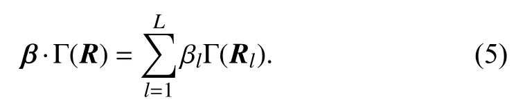
The regularization term Γ(R) guarantees that the solution accords with the degradation process of the minimization of(4). It is determined by a specified noise distribution. For example, when considering the Gaussian noise estimation, we use an ?2-norm regularization term:

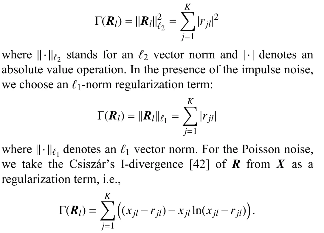
For a common single noise, i.e., Gaussian, Poisson, and impulse noise, the above regularization terms lead to a maximum a posteriori (MAP) solution to such noise estimation. In real-world applications, images are generally contaminated by mixed or unknown noise rather than a single noise. The regularization terms for single noise estimation become inapplicable since the distribution of mixed or unknown noise is difficult to be modeled mathematically.Therefore, one of this work’s purposes is to design a universal regularization term for mixed or unknown noise estimation.

D. Analysis of Mixed Noise Distribution

To reveal the essence of mixed noise distributions, we here consider generic and representative mixed noise, i.e., a mixture of Poisson, Gaussian, and impulse noise. Let us take an example to exhibit its distribution. Here, we impose Gaussian noise (σ =10) and a mixture of Poisson, Gaussian(σ =10 ) and random-valued impulse noise ( p=20%) on image Lena with size 512×512, respectively. We show original and two observed images in Fig.2.

As Fig.2(b) shows, Gaussian noise is overall orderly. As a common sense, Poisson distribution is a Gaussian-like one under the condition of having enough samples. Therefore, due to impulse noise, mixed noise is disordered and unsystematic as shown in Fig.2(c). In Fig.3, we portray the distributions of Gaussian and mixed noise, respectively.

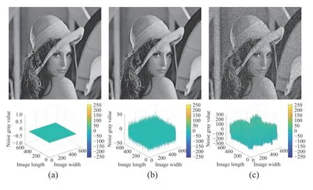
Fig.2. Noise-free image and two observed ones corrupted by Gaussian and mixed noise, respectively. The first row: (a) noise-free image; (b) observed image with Gaussian noise; and (c) observed image with mixed noise. The second row portrays noise included in three images.

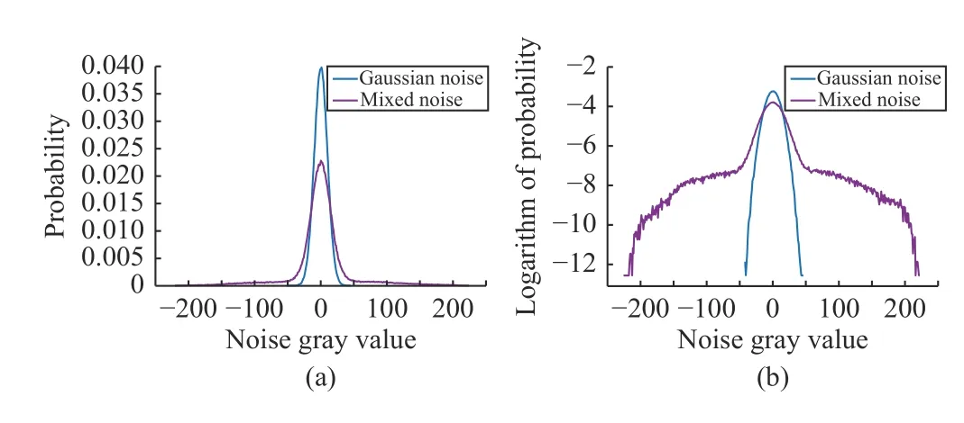
Fig.3. Distributions of Gaussian and mixed noise in different domains. (a)linear domain; and (b) logarithmic domain.

Fig.3(a) shows noise distribution in a linear domain. To intuitively illustrate a heavy tail, we present it in a logarithmic domain as shown in Fig.3(b). Clearly, Poisson noise leads to a Gaussian-like distribution. Nevertheless, impulse noise gives rise to a more irregular distribution with a heavy tail.Therefore, neither ?1nor ?2norm can precisely characterize residual R in the sense of MAP estimation.

E. Residual-driven FCM With Weighted ?2-norm Regularization

Intuitively, if the regularization term can be modified so as to make mixed noise distribution more Gaussian-like, we can still use ?2norm to characterize residual R. It means that mixed noise can be more accurately estimated. Therefore, we adopt robust estimation techniques [43], [44] to weaken the heavy tail, which makes mixed noise distribution more regular. In the sequel, we assign a proper weight wjlto each residual rjl, which forms a weighted residual wjlrjlthat almost obeys a Gaussian distribution. Given Fig.4, we use an example for showing the effect of weighting.

Fig.4(a) shows the distribution of rjland the fitting Gaussian function based on the variance of rjl. Fig.4(b) gives the distribution of wjlrjland the fitting Gaussian function based on the variance of wjlrjl. Clearly, the distribution of wjlrjlin Fig.4(b) is more Gaussian-like than that in Fig.4(a), which means that ?2-norm regularization can work on weighted residual wjlrjlfor an MAP-like solution of R.

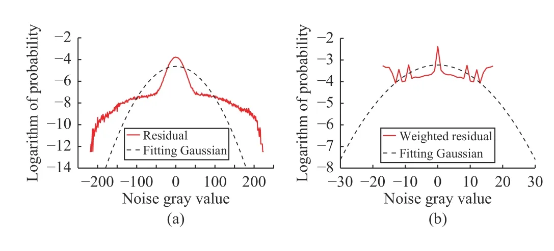
Fig.4. Distributions of residual rjl and weighted residual wjlrjl, as well as the fitting Gaussian function in the logarithmic domain.

By analyzing Fig.4, for l=1,2,...,L, we propose a weighted ?2-norm regularization term for mixed or unknown noise estimation:

where ξ is a positive parameter, which aims to control the decreasing rate of wjl.

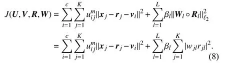
By substituting (6) into (4) combined with (5), we present RFCM with weighted ?2-norm regularization (WRFCM) for image segmentation:

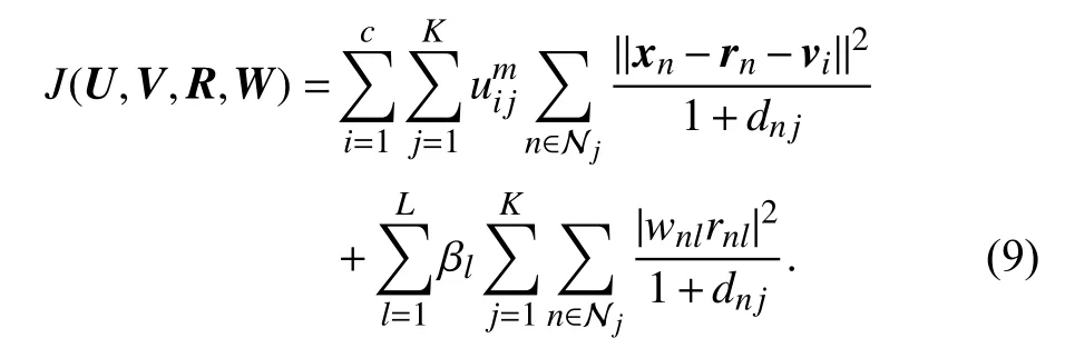
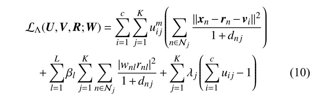
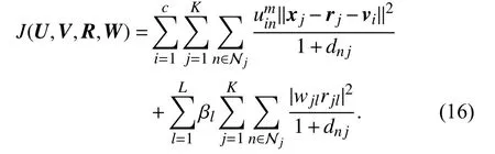
When coping with image segmentation problems, since each image pixel is closely related to its neighbors, using spatial information has a positive impact on FCM as shown in [9],[34]. If there exists a small distance between a target pixel and its neighbors, they most likely belong to a same cluster.Therefore, we introduce spatial information into (8), thus resulting in our final objective function:

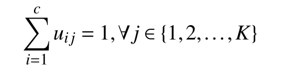
Its minimization is completed subject to

In (9), an image pixel is sometimes loosely represented by its corresponding index even though this is not ambiguous.Thus, n is a neighbor pixel of j and dnjrepresents the Euclidean distance between n and j . Njstands for a local window centralized at j including j and its size is | Nj|.

F. Minimization Algorithm

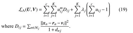
Minimizing (9) involves four unknowns, i.e., U, V , R and W. According to (7), W is automatically determined by R.Hence, we can design a two-step iterative algorithm to minimize (9), which fixes W first to solve U, V and R, then uses R to update W. The main task in each iteration is to solve the minimization problem in terms of U, V and R when fixing W. Assume that W is given. We can apply a Lagrangian multiplier method to minimize (9). The Lagrangian function is expressed as

where Λ={λj: j=1,2,...,K} is a set of Lagrangian multipliers. The two-step iterative algorithm for minimizing(9) is realized in Algorithm 1.

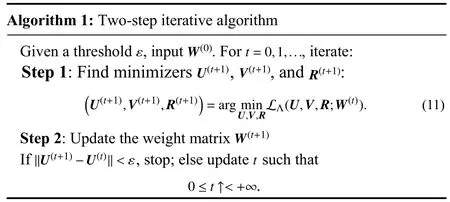
The minimization problem (11) can be divided into the following three subproblems:

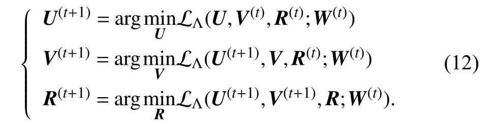
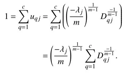
Each subproblem in (12) has a closed-form solution. We use an alternative optimization scheme similar to the one used in FCM to optimize U and V. The following result is needed to obtain the iterative updates of U and V.

Theorem 1: Consider the first two subproblems of (12). By applying the Lagrangian multiplier method to solve them, the iterative solutions are presented as

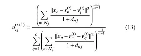
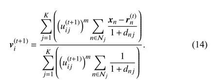
Proof: See the Appendix ■

In the last subproblem of (12), both rjand rnappear simultaneously. Since rnis dependent on rj, it should not be considered as a constant vector. In other words, n is one of neighbors of j while j is one of neighbors of n symmetrically.Thus, n ∈Njis equivalent to j ∈Nn. Then we have

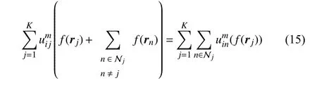
where f represents a function in terms of rjor rn. By (15), we rewrite (9) as

According to the two-step iterative algorithm, we assume that W in (16) is fixed in advance. When U and V are updated, the last subproblem of (12) is separable and can be decomposed into K×L subproblems:

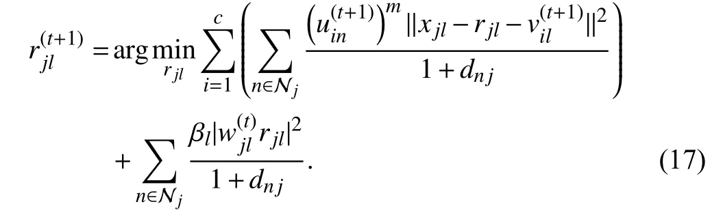
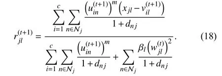
By zeroing the gradient of the energy function in (17) in terms of rjl, the iterative solution to (17) is expressed as

To quantify the impact of weighted ?2-norm regularization on FCM, we show an example, as shown in Fig.5. We impose a mixture of Poisson, Gaussian, and impulse noise (σ=30,p=20%) on a noise-free image in Fig.5(a). We set c to 4.The settings of ξ and β are discussed in the later section.

As shown in Fig.5, the noise estimation of DSFCM_N in Fig.5(g) is far from the true one in Fig.5(f). However,WRFCM achieves a better noise estimation result as shown in Fig.5(h). In addition, it has better performance for noisesuppression and feature-preserving than DSFCM_N, which can be visually observed from Figs. 5(c) and (d).

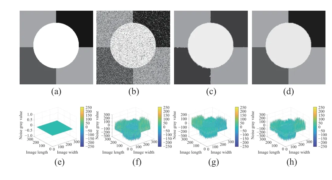
Fig.5. Noise estimation comparison between DSFCM_N and WRFCM. (a)noise-free image; (b) observed image; (c) segmented image of DSFCM_N;(d) segmented image of WRFCM; (e) noise in the noise-free image; (f) noise in the observed image; (g) noise estimation of DSFCM_N; and (h) noise estimation of WRFCM.

Algorithm 2: Residual-driven FCM with weighted -norm regularization (WRFCM)?2 Input: Observed image , fuzzification exponent , number of clusters , and threshold .^X Xmc ε Output: Segmented image .W(0) 1 V(0)1: Initialize as a matrix with all elements of and generate randomly prototypes t ←0 2: 3: repeat U(t+1)4: Calculate the partition matrix via (13)V(t+1)5: Calculate the prototypes via (14)6: Calculate the residual via (18)R(t+1)W(t+1)7: Update the weight matrix via (7)t ←t+1 8: ‖U(t+1)?U(t)‖<ε 9: until 10: return , , and UV R W 11: Generate the segmented image based on and ^X U V

G. Convergence and Robustness Analysis

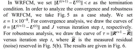
As Fig.6(a) indicates, since the prototypes are randomly initialized, WRFCM oscillates slightly at the beginning.Nevertheless, it reaches steady state after a few iterations.Even though θ exhibits some oscillation, the objective function value J keeps decreasing until the iteration stops.Affected by the oscillation of θ , τ takes on a pattern of increasing and then decreasing and eventually stabilizes. The finding indicates that WRFCM can obtain optimal residual estimation as t increases. To sum up, WRFCM has outstanding convergence and robustness since the weight ?2-norm regularization makes mixed noise distribution estimated accurately so that the residual is gradually separated from observed data as iterations proceed.

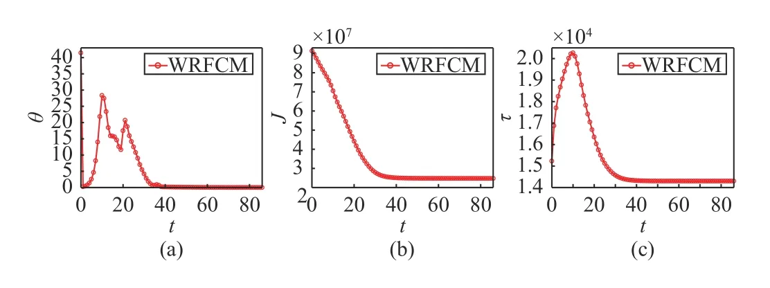
Fig.6. Convergence and robustness of WRFCM. (a) θ ; (b) J ; and (c) τ versus t.

III. EXPERIMENTAL STUDIES

In this section, to show the performance, efficiency and robustness of WRFCM, we provide numerical experiments on synthetic, medical, and other real-world images. To highlight the superiority and improvement of WRFCM over conventional FCM, we also compare it with seven FCM variants, i.e., FCM_S1 [10], FCM_S2 [10], FLICM [13],KWFLICM [15], FRFCM [30], WFCM [22], and DSFCM_N[34]. They are the most representative ones in the field. At the last of this section, to further verify WRFCM’s strong robustness, we compare WRFCM with two competing approaches unrelated to FCM, i.e., PFE [45] and AMR_SC[46]. For a fair comparison, we note that all experiments are implemented in Matlab on a laptop with Intel(R) Core(TM)i5-8250U CPU of (1.60 GHz) and 8.0 GB RAM.

A. Evaluation Indicators

To quantitatively evaluate the performance of WRFCM, we adopt three objective evaluation indicators, i.e., segmentation accuracy (SA) [15], Matthews correlation coefficient (MCC)[47], and Sorensen-Dice similarity (SDS) [48], [49]. Note that a single one cannot fully reflect true segmentation results. SA is defined as

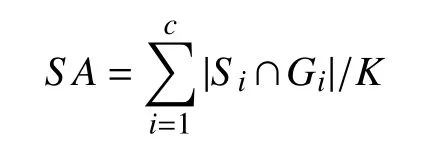
where Siand Giare the i-th cluster in a segmented image and its ground truth, respectively. |·| denotes the cardinality of a set. MCC is computed as

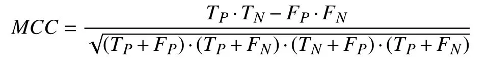
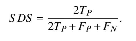
where TP, FP, TN, and FNare the numbers of true positive,false positive, true negative, and false negative, respectively.SDS is formulated as

B. Dataset Descriptions

Tested images except for synthetic ones come from five publicly available databases including a medical one and four real-world ones. The details are outlined as follows:

1) BrianWeb: This is an online interface to a 3D MRI simulated brain database. The parameter settings are fixed to 3 modalities, 5 slice thicknesses, 6 levels of noise, and 3 levels of intensity non-uniformity. BrianWeb provides golden standard segmentation.

2) Berkeley Segmentation Data Set (BSDS) [50]: This database contains 200 training, 100 validation and 200 testing images. Golden standard segmentation is annotated by different subjects for each image of size 321×481 or 481×321.

3) Microsoft Research Cambridge Object Recognition Image Database (MSRC): This database contains 591 images and 23 object classes. Golden standard segmentation is provided.

4) NASA Earth Observation Database (NEO): This database continually provides information collected by NASA satellites about Earth’s ocean, atmosphere, and land surfaces. Due to bit errors appearing in satellite measurements, sampled images of size 1440×720 contain unknown noise. Thus, their ground truths are unknown.

5) PASCAL Visual Object Classes 2012 (VOC2012): This dataset contains 20 object classes. The training/validation data has 11 530 images containing 27 450 ROI annotated objects and 6929 segmentations. Each image is of size 500×375 or 375×500.

C. Parameter Settings

where δlis the standard deviation of the l- th channel of X . If ? is set, βlis computed. Therefore, β is equivalently replaced by ?. In Fig.7, we cover an example to show the setting of ? associated with Fig.8.

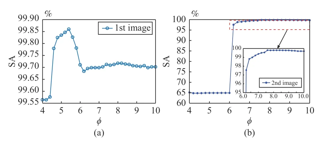
Fig.7. SA values versus ?.

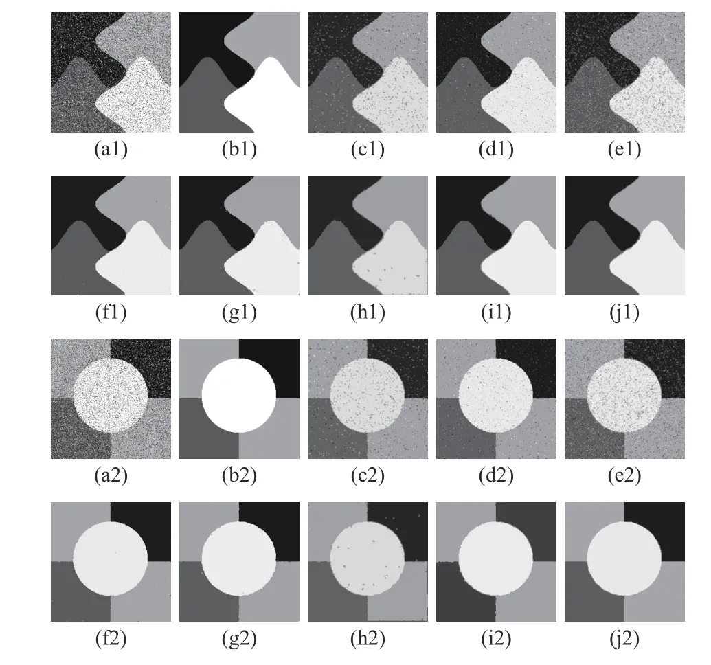
Fig.8. Visual results for segmenting synthetic images ( ?1=5.58 and ?2=7.45). From (a1) to (j1) and from (a2) to (j2): noisy images, ground truth,and results of FCM_S1, FCM_S2, FLICM, KWFLICM, FRFCM, WFCM,DSFCM_N, and WRFCM.

As Fig.7(a) indicates, when coping with the first image, the SA value reaches its maximum gradually as the value of ? increases. Afterwards, it decreases rapidly and tends to be stable. As shown in Fig.7(b), for the second image, after the SA value reaches its maximum, it has no apparent changes,implying that the segmentation performance is rather stable.In conclusion, for image segmentation, WRFCM can produce better and better performance as parameter ? increases from a small value.

D. Experimental Results and Analysis

We show the comparison results between WRFCM and seven FCM-related algorithms. We test a set of synthetic,medical, and real-world images. They are borrowed from four public datasets, i.e., BrainWeb, BSDS, MSRC, and NEO.

1) Results on Synthetic Images: In the first experiment, we representatively choose two synthetic images of size 256×256. A mixture of Poisson, Gaussian, and impulse noises is considered for all cases. To be specific, Poisson noise is first added. Then we add Gaussian noise with σ=30.Finally, the random-valued impulse noise with p=20% is added since it is more difficult to detect than salt and pepper impulse noise. For two images, we set c=4. The segmentation results are given in Fig.8 and Table I. The best values are in bold.

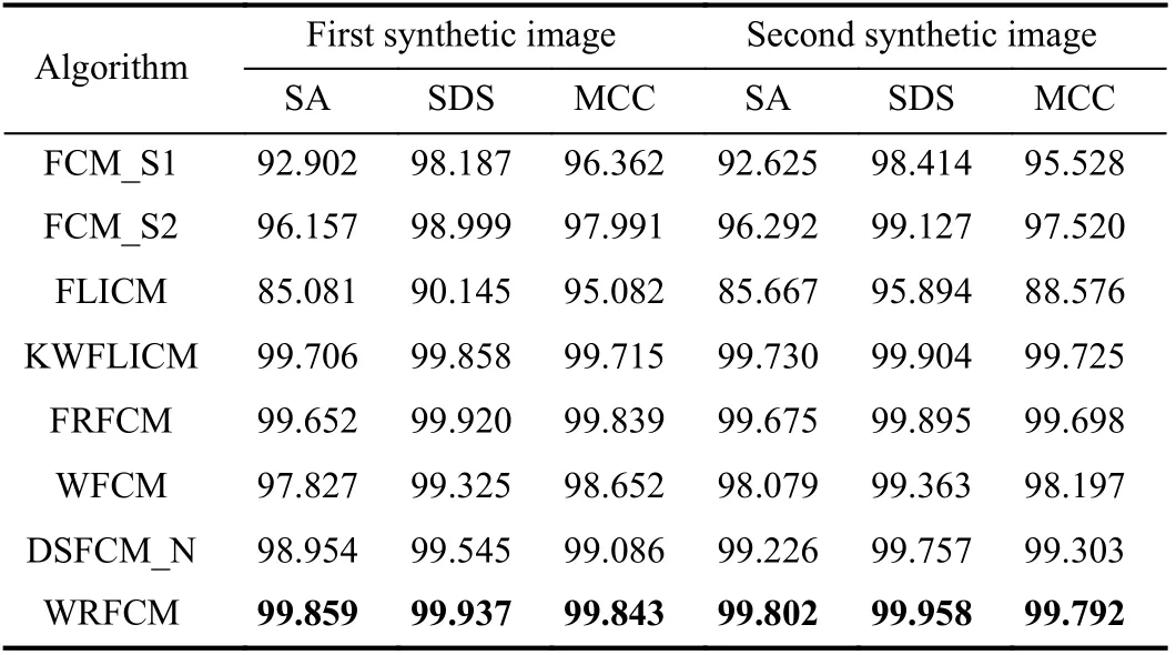
TABLE I SEGMENTATION PERFORMANCE (%) ON SYNTHETIC IMAGES

As Fig.8 indicates, FCM_S1, FCM_S2 and FLICM achieve poor results in presence of such a high level of mixed noise.Compared with them, KWFLICM, FRFCM and WFCM suppress the vast majority of mixed noise. Yet they cannot completely remove it. DSFCM_N visually outperforms other peers mentioned above. However, it generates several topology changes such as merging and splitting. By taking the second synthetic image as a case, we find that DSFCM_N produces some unclear contours and shadows. Superiorly to seven peers, WRFCM not only removes all the noise but also preserves more image features.

Table I shows the segmentation results of all algorithms quantitatively. It assembles the values of all three indictors.Clearly, WRFCM achieves better SA, SDS, and MCC results for all images than other peers. In particular, its SA value comes up to 99.859% for the first synthetic image. Among its seven peers, KWFLICM obtains generally better results. In the light of Fig.8 and Table I, we conclude that WRFCM performs better than its peers.

2) Results on Medical Images: Next, we representatively segment two medical images from BrianWeb. They are represented as two slices in the axial plane with 70 and 80,which are generated by T1 modality with slice thickness of 1mm resolution, 9% noise and 20% intensity non-uniformity.Here, we set c=4 for all cases. The comparisons between WRFCM and its peers are shown in Fig.9 and Table II. The best values are in bold.

By viewing the marked red squares in Fig.9, we find that FCM_S1, FCM_S2, FLICM, KWFLICM and DSFCM_N are vulnerable to noise and intensity non-uniformity. They give rise to the change of topological shapes to some extent. Unlike them, FRFCM and WFCM achieve sufficient noise removal.However, they produce overly smooth contours. Compared with its seven peers, WRFCM can not only suppress noise adequately but also acquire accurate contours. Moreover, it yields the visual result closer to ground truth than its peers. As Table II shows, WRFCM obtains optimal SA, SDS and MCC results for all medical images. As a conclusion, it outperforms its peers visually and quantitatively.

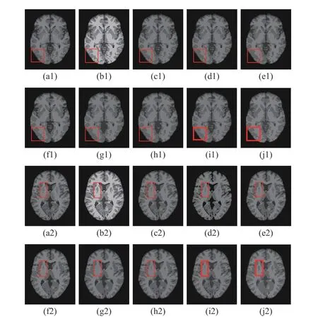
Fig.9. Visual results for segmenting medical images (? =5.35). From (a1)to (j1) and from (a2) to (j2): noisy images, ground truth, and results of FCM_S1, FCM_S2, FLICM, KWFLICM, FRFCM, WFCM, DSFCM_N, and WRFCM.

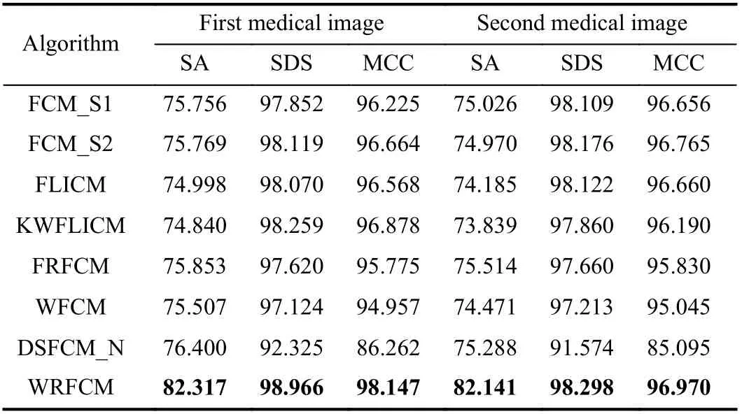
TABLE II SEGMENTATION PERFORMANCE (%) ON MEDICAL IMAGES IN BRIANwEB

3) Results on Real-world Images: In order to demonstrate the practicality of WRFCM for other image segmentation, we typically choose two sets of real-world images in the last experiment. The first set contains five representative images from BSDS and MSRC. There usually exist some outliers,noise or intensity inhomogeneity in each image. For all tested images, we set c=2. The results of all algorithms are shown in Fig.10 and Table III.

Fig.10 visually shows the comparison between WRFCM and seven peers while Table III gives the quantitative comparison. Apparently, WRFCM achieves better segmentation results than its peers. FCM_S1, FCM_S2, FLICM,KWFLICM and DSFCM_N obtain unsatisfactory results on all tested images. Superiorly to them, FRFCM and WFCM

preserve more contours and feature details. From a quantitative point of view, WRFCM acquires optimal SA,SDS, and MCC values much more than its peers. Note that it merely gets a slightly smaller SDS value than FRFCM and WFCM for the first and second images, respectively.

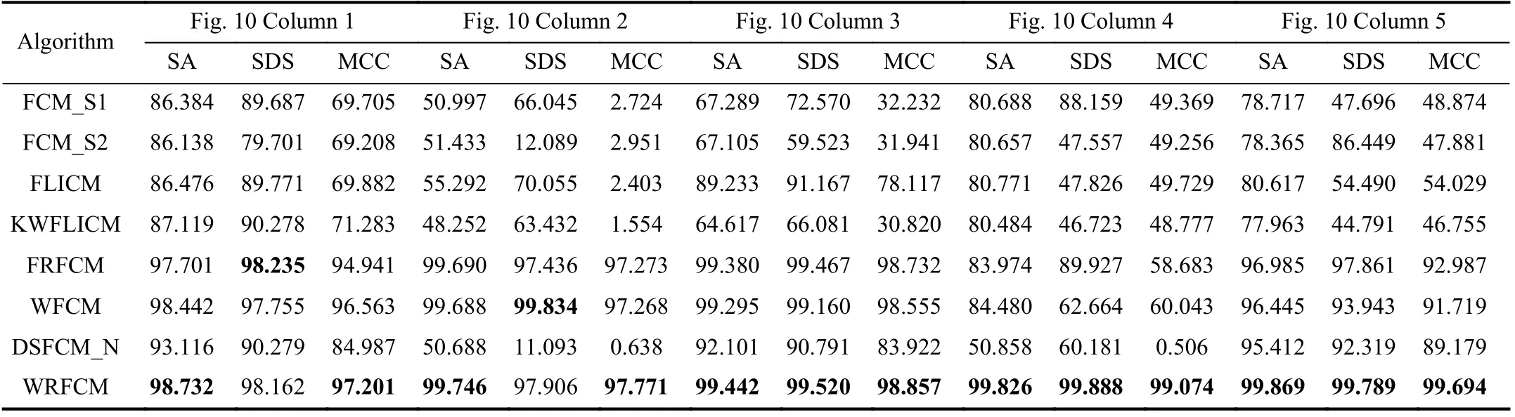
TABLE III SEGMENTATION PERFORMANCE (%) ON REAL-wORLD IMAGES IN BSDS AND MSRC

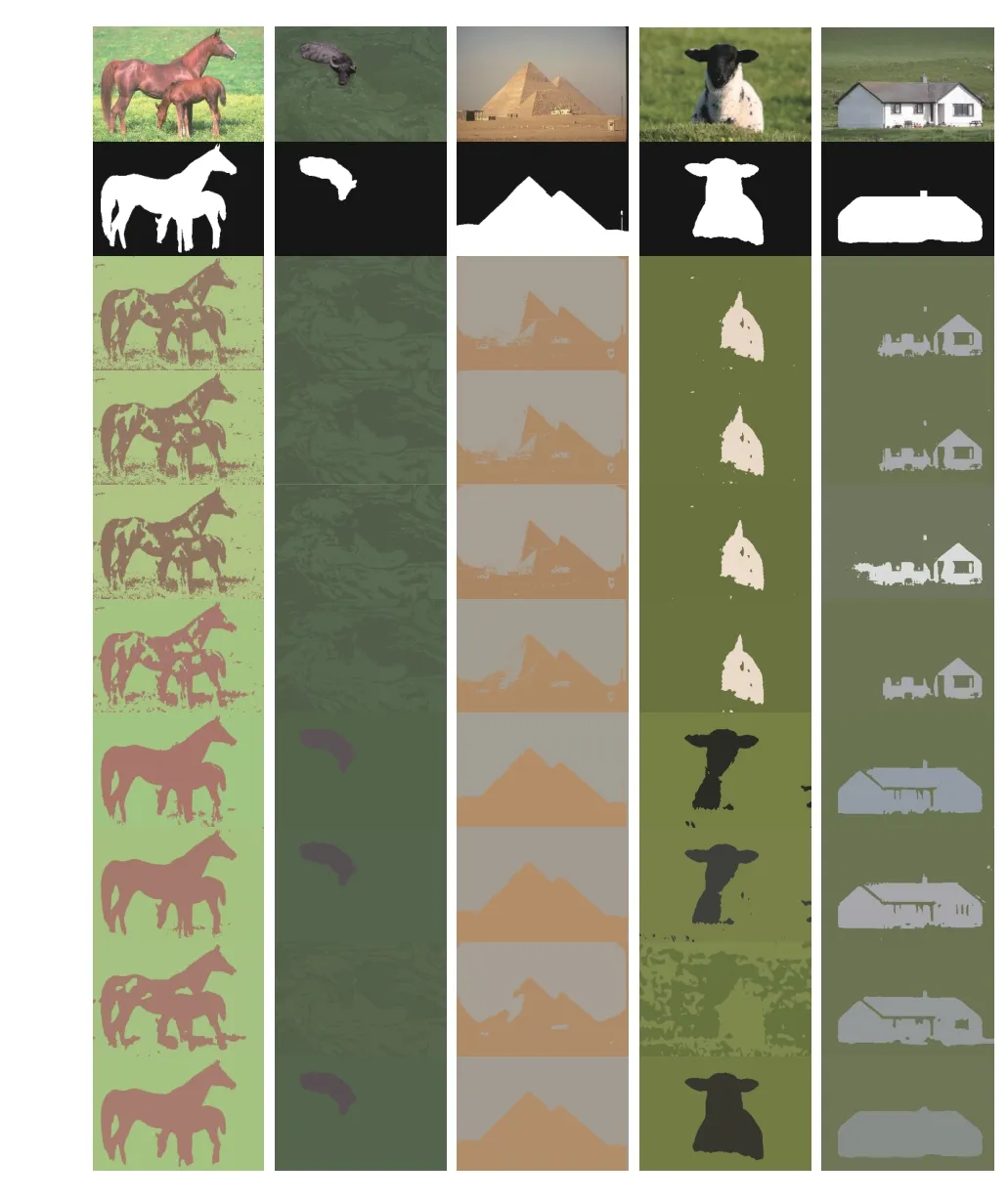
Fig.10. Segmentation results on five real-world images in BSDS and MSRC (? 1=6.05, ?2=10.00 , ?3=9.89 , ?4=9.98, and ?5=9.50). From top to bottom: observed images, ground truth, and results of FCM_S1, FCM_S2,FLICM, KWFLICM, FRFCM, WFCM, DSFCM_N, and WRFCM.

The second set contains images from NEO. Here, we select two typical images. Each of them represents an example for a specific scene. We produce the ground truth of each scene by randomly shooting it for 50 times within the time span 2000–2019. The visual results of all algorithms are shown in Figs. 11 and 12. The corresponding SA, SDS, and MCC values are given in Table IV.

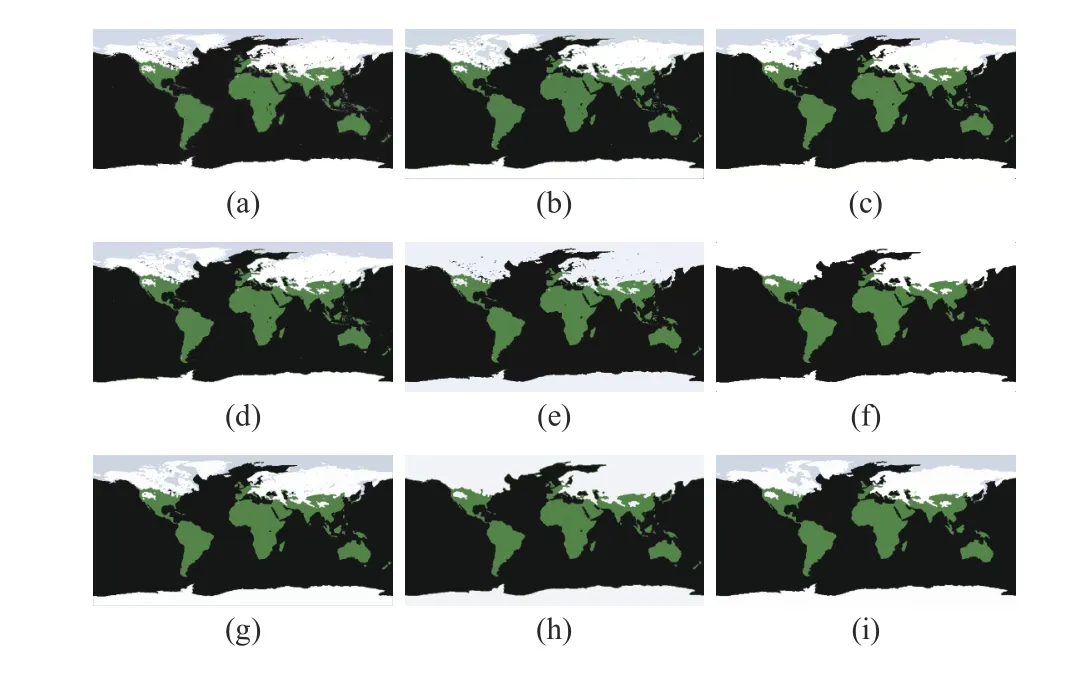
Fig.11. Segmentation results on the first real-world image in NEO(? =6.10). From (a) to (i): observed image and results of FCM_S1, FCM_S2,FLICM, KWFLICM, FRFCM, WFCM, DSFCM_N, and WRFCM.

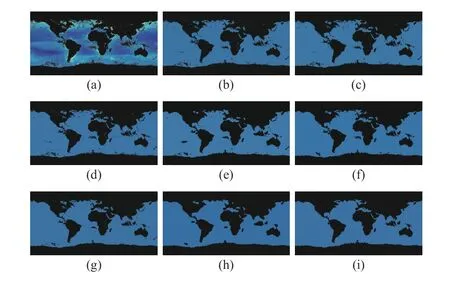
Fig.12. Segmentation results on the second real-world image in NEO(? =9.98). From (a) to (i): observed image and results of FCM_S1, FCM_S2,FLICM, KWFLICM, FRFCM, WFCM, DSFCM_N, and WRFCM.

Fig.11 shows the segmentation results on sea ice and snow extent. The colors represent the land and ocean covered by snow and ice per week (here is February 7–14, 2015). We set c=4. Fig.12 gives the segmentation results on chlorophyll concentration. The colors represent where and how much phytoplankton is growing over a span of days. We choose c=2. As a whole, by seeing Figs. 11 and 12, as well as Table IV, FCM_S1, FCM_S2, FLICM, KWFLICM, and WFCM are sensitive to unknown noise. FRFCM and DSFCM_N produce overly smooth results. Especially, they generate incorrect clusters when segmenting the first image inNEO. Superiorly to its seven peers, WRFCM cannot only suppress unknown noise well but also retain image contours well. In particular, it makes up the shortcoming that other peers forge several topology changes in the form of black patches when coping with the second image in NEO.

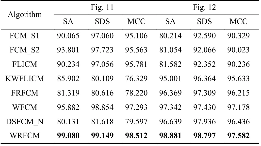
TABLE IV SEGMENTATION PERFORMANCE (%) ON REAL-wORLD IMAGES IN NEO

4) Performance Improvement: Besides segmentation results reported for all algorithms, we also present the performance improvement of WRFCM over seven comparative algorithms in Table V. Clearly, for all types of images, the average SA,SDS and MCC improvements of WRFCM over other peers are within the value span 0.113%–27.836%, 0.040%–41.989%,and 0.049%–58.681%, respectively.

TABLE V AVERAGE PERFORMANCE IMPROVEMENTS (%) OF WRFCM OVER COMPARATIVE ALGORITHMS

5) Overhead Analysis: In the previous subsections, the segmentation performance of WRFCM is presented. Next, we provide the comparison of computing overheads between WRFCM and seven comparative algorithms in order to show its practicality. We note that K is the number of image pixels,c is the number of prototypes, t is the iteration count, ω represents the size of a filtering window, |Nj| denotes the size of a local window centralized at pixel j , and μ is the number of pixel levels in an image. Generally, μ?K. Generally speaking, since FCM-related algorithms are unsupervised and their solutions are easily updated iteratively, they have low storage complexities of O(K). In addition, we summarize the computational complexity of all algorithms in Table VI.

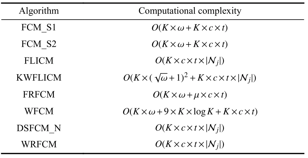
TABLE VI COMPUTATIONAL COMPLEXITY OF ALL ALGORITHMS

As Table VI shows, FRFCM has lower computational complexity than its peers since μ?K. Except WFCM, the complexity of other algorithms is basically O(K), and that of WRFCM is not high. To compare the practicability between WRFCM and its peers, we present the execution time of all algorithms for segmenting synthetic, medical, and real-world images in Table VII.

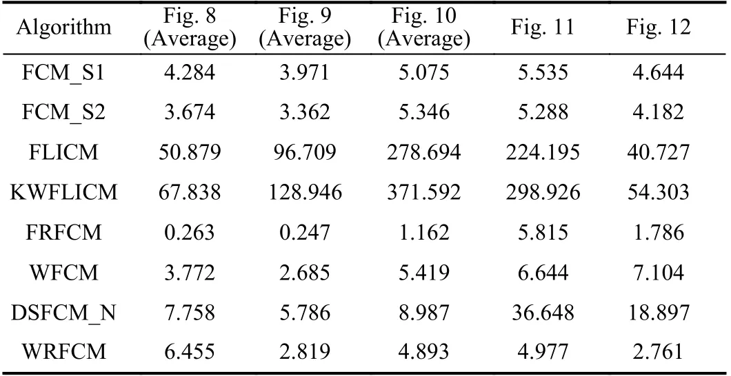
TABLE VII COMPARISON OF EXECUTION TIME (IN SECONDS) OF ALL ALGORITHMS

As Table VII shows, for gray and color image segmentation,the computational efficiencies of FLICM and KWFLICM are far lower than those of others. In contrast, since gray level histograms are considered, FRFCM takes the least execution time among all algorithms. Due to the computation of a neighbor term in advance, FCM_S1 and FCM_S2 are more time-saving than most of other algorithms. Even though WFCM and DSFCM_N need more computing overheads than FRFCM, they are still very efficient. For color image segmentation, the execution time of DSFCM_N increases dramatically. Compared with most of seven comparative algorithms, WRFCM shows higher computational efficiency.In most cases, it only runs slower than FRFCM. However, the shortcoming can be offset by its better segmentation performance. In a quantitative study, for each image,WRFCM takes 0.011 s and 2.642 s longer than FCM_S2 and FRFCM, respectively. However, it saves 0.321 s, 133.860 s,179.940 s, 0.744 s, and 11.234 s over FCM_S1, FLICM,KWFLICM, FRFCM, WFCM, and DSFCM_N, respectively.

E. Comparison With Non-FCM Methods

We compare WRFCM with two non-FCM methods, i.e.,PFE [45] and AMR_SC [46]. We list the comparison results on VOC2012 in Fig.13 and Table VIII. The computing times of the WRFCM, AMR_SC, and PFE are summarized in Table IX.The results indicate that WRFCM achieves better effectiveness and efficiency than AMR_SC and PFE.

Fig.13. Segmentation results on four real-world images in VOC2012( ?1=5.65, ? 2=6.75, ? 3=5.50 , ? 4=8.35). From top to bottom: observed images, ground truth, and results of AMR_SC, PFE, and WRFCM.

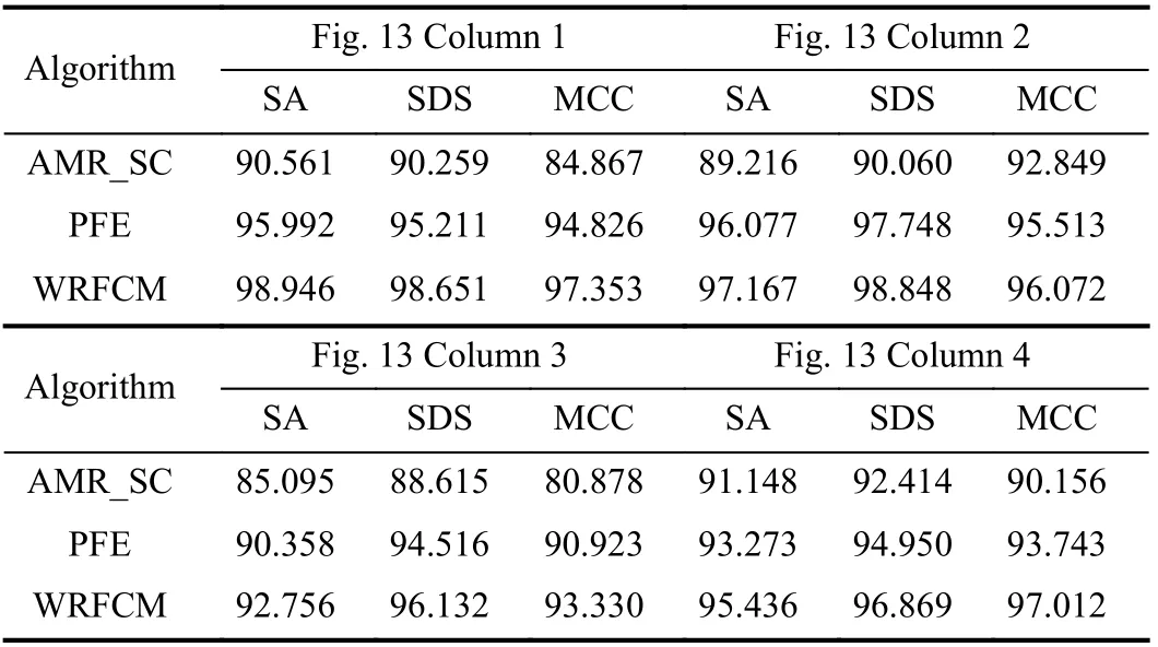
TABLE VIII SEGMENTATION PERFORMANCE (%) ON REAL-wORLD IMAGES IN VOC2012

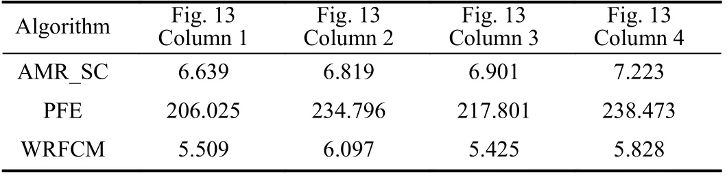
TABLE IX COMPARISON OF EXECUTION TIME (IN SECONDS)

IV. CONCLUSIONS AND FUTURE WORK

For the first time, a residual-driven Fuzzy C-Means (RFCM)framework is proposed for image segmentation, which advances FCM research. It realizes favorable noise estimation in virtue of a residual-related regularization term coming with an analysis of noise distribution. On the basis of the framework, RFCM with weighted ?2-norm regularization (WRFCM) is presented for coping with image segmentation with mixed or unknown noise. Spatial information is also considered in WRFCM for making residual estimation more reliable. A two-step iterative algorithm is presented to implement WRFCM. Experimental results reported for four benchmark databases show that it outperforms existing FCM and non-FCM methods. Moreover, differing from residuallearning methods, it is unsupervised and exhibits high speed clustering.

There are some open issues worth pursuing. First, since a tight wavelet frame transform [51]–[53] provides redundant representations of images, it can be used to manipulate and analyze image features and noise well. Therefore, it can be taken as a kernel function so as to produce an improved FCM algorithm, i.e., wavelet kernel-based FCM. Second, can the proposed algorithm be applied to a wide range of non-flat domains such as remote sensing [54], ecological systems [55],feature recalibration network [56], and 3D images [57]? How can the number of clusters be selected automatically? Can more recently proposed minimization algorithms [58]–[61] be applied to the optimization problem involved in this work?Answering them needs more efforts.

APPENDIX

PROOF OF THEOREM 1

Proof: Consider the first two subproblems of (12). The Lagrangian function (10) is reformulated as

By fixing V, we minimize (19) in terms of U. By zeroing the gradient of (19) in terms of U, one has

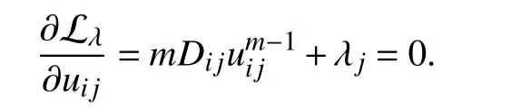
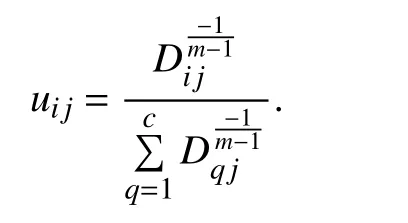
Thus, uijis expressed as

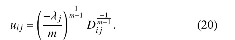
In the sequel, one can get

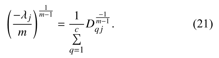
Substituting (21) into (20), the optimal uijis acquired:

By fixing U, we minimize (19) in terms of V. By zeroing the gradient of (19) in terms of V, one has

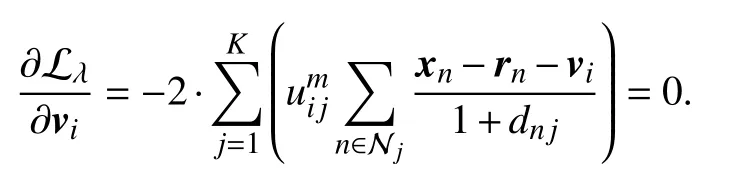
The intermediate process is presented as

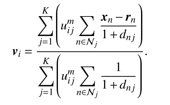
The optimal viis computed: