OPTIMAL CONTROL PROBLEMFOR EXACT SYNCHRONIZATION OF ORDINARY DIFFERENTIAL SYSTEMS
2019-05-25 03:57:02WUKefan
數(shù)學(xué)雜志 2019年3期
WU Ke-fan
(School of Mathematics and Statistics,Wuhan University,Wuhan 430072,China)
Abstract: In this paper,we study a kind of optimal problems related to the exact synchronization for a controlled linear ordinary dif f erential system.We establish a necessary and sufficient condition for the optimal control.Moreover,we give the numerical approximation of the optimal control and present some examples to test the ef f ectiveness of the algorithm.
Keywords: exact synchronization;necessary and sufficient conditions;ordinary dif f erential system;numerical approximation
1 Introduction
1.1 Background
Synchronization is a widespread natural phenomenon.It was first observed by Huygens in 1967[1].For instance,pacemaker cells of the heart function simultaneously;thousands of firef l ies may twinkle at the same time;audiences in the theater can applaud with a rhythmic beat;and field crickets give out a unanimous cry[2–4].The theoretical studies on synchronization phenomena from the perspective of mathematics were started by Wiener in the 1950s[5].
Mathematically,the exact synchronization for a controlled system is to ask for a control so that the dif f erence of any two components of the corresponding solution to the system(with an initial state)takes value zero at a fixed time and remains the value zero after the aforementioned fixed time.The exact synchronization in the PDEs case was first studied for a coupled system of wave equations both for the higher-dimensional case in the framework of weak solutions in[6–8],and for the one-dimensional case in the framework of classical solutions in[2]and[9].A minimal time control problem for the exact synchronization of some parabolic systems was studied in[10].
In this paper,we consider an optimal control problem related to the exact synchronization for a kind of linear ordinary dif f erential system.
1.2 Formulation of the Problem and Hypotheses
Let A∈ Rn×nand B ∈Rn×mbe two constant matrices,where n≥ 2 and m ≥ 1.Let y0∈Rn.Consider the following controlled linear ordinary dif f erential system
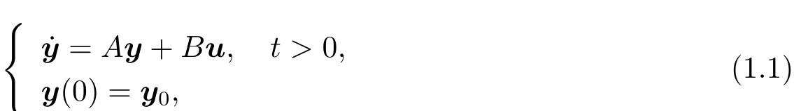
where u∈L2(0,+∞;Rm)is a control.Write

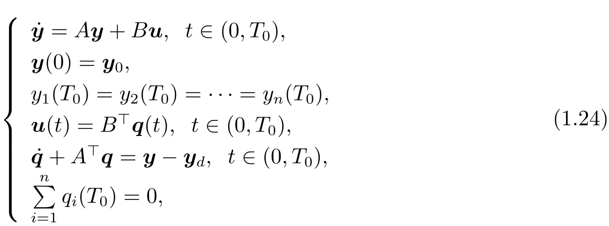
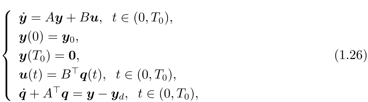
for the solution of(1.1).Here and throughout this paper,we denote the transposition of a matrix J by J>.It is well known that for each T>0,y(·;y0,u) ∈ C([0,T];Rn).Given T0>0,y0∈Rnand yd∈L2(0,T0;Rn),we define an optimal control problem as follows
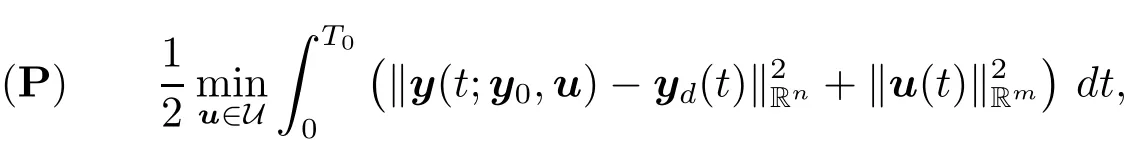
where
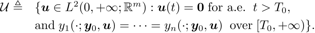
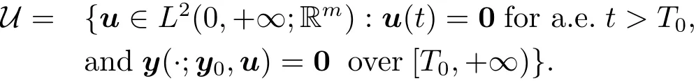
Two concepts related to this problem are the null controllability and the exact synchronization.Let us recall them.First,the system(1.1)is said to be null controllable at time T,if for any y0∈Rn,there exists a control u∈L2(0,+∞;Rm)with u(t)=0 over(T,+∞),so that y(t;y0,u)=0 for all t≥T.Second,the system(1.1)is said to be exactly synchronizable at time T,if for any y0∈Rn,there exists a control u∈L2(0,+∞;Rm)with u(t)=0 over(T,+∞),so that

Mathematically,the exact synchronization is weaker than the null controllability.
Here and throughout this paper,we denote A=(aij)1≤i,j≤n,B=(bij)1≤i≤n,1≤j≤mand
We shall use h·,·i to denote the inner product of Rnor Rmif there is no risk of causing any confusion.
In this paper,we assume that A and B satisfy the following hypothesis(H1)or(H2).
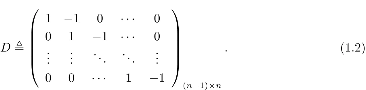
(H1)The pair(A,B)satisfies that
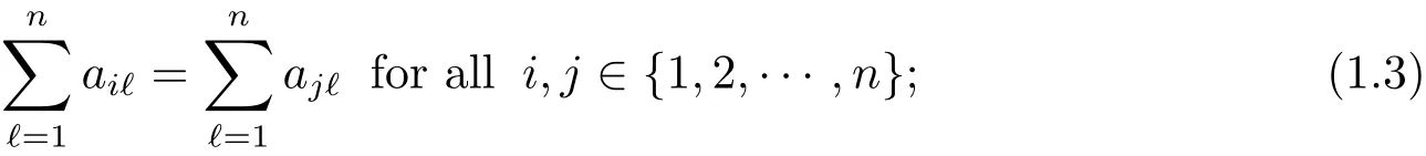
and that rank(DB,DAB,···,DAn?2B)=n ? 1.Recall that D is given by(1.2).
(H2)The pair(A,B)satis fies that
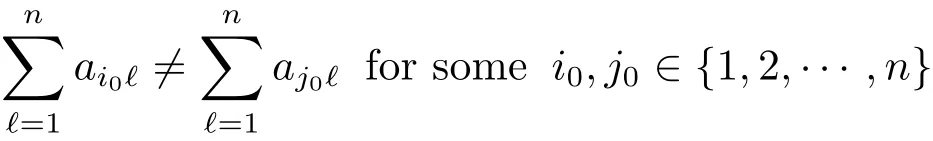
and that

The main result of this paper is as follows.
Theorem 1.1Suppose that A and B satisfy either(H1)or(H2).Then problem(P)has a unique optimal control.Moreover,
(i)If A and B satisfy(H1),u?is the optimal control to problem(P)if and only if u?∈U and there exists a function q∈C([0,T0];Rn)so that

and
(ii)If A and B satisfy(H2),u?is the optimal control to problem(P)if and only if u?∈U and there exists a function q∈C([0,T0];Rn)so that

and

where y?is the solution to(1.1)corresponding to the optimal control u?,i.e.,y?(·)=y(·;y0,u?).
Pontryagin’s maximum principle of optimal control problems for dif f erential equations was studied for decades[11–15]and the references therein.Recently,Pontryagin’s maximum principle of optimal control problems for the exact synchronization of the parabolic dif f erential equations was considered in[16].However,the sufficient condition for the abovementioned problem was not derived in[16].This paper is organized as follows.In Section 2,we prove Theorem 1.1.In Section 3,we give the numerical approximation of the optimal control and present some examples to test the ef f ectiveness of the algorithm.
2 Proof of Theorem 1.1
Under hypothesis(H1)or(H2),by the same arguments as those in[16],we can show the existence and uniqueness of the optimal control of problem(P).We omit the proofs here.Next,we continue the proof of Theorem 1.1.
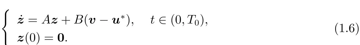
(i)We start with the proof of“Necessity” part.For any v ∈ U and λ ∈ (0,1),we set uλ,u?+λ(v?u?).Then uλ∈ U.Denote

We can show that
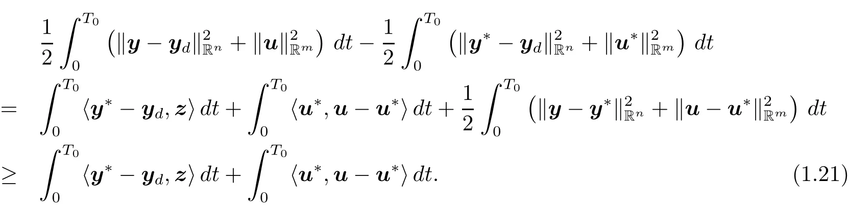
Since u?is the optimal control to problem(P),we get
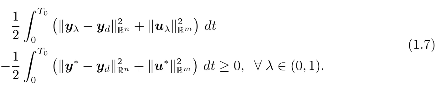
Dividing by λ and passing to the limit for λ → 0+in(1.7),we have
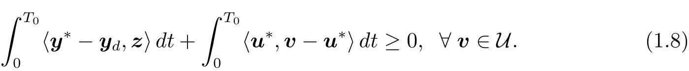
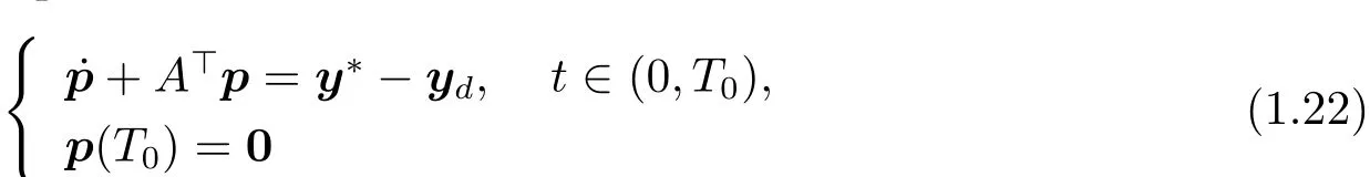
Let p be the solution to the following system
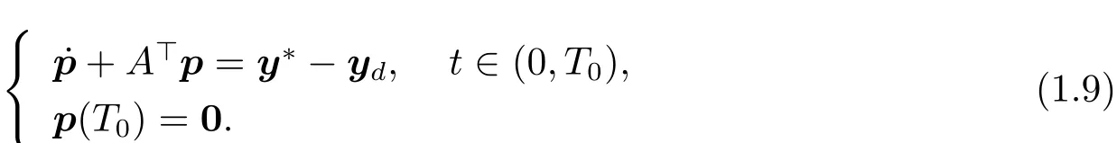
Multiplying the first equation of(1.9)by z and integrating it over(0,T0),by(1.6)and(1.9),we get
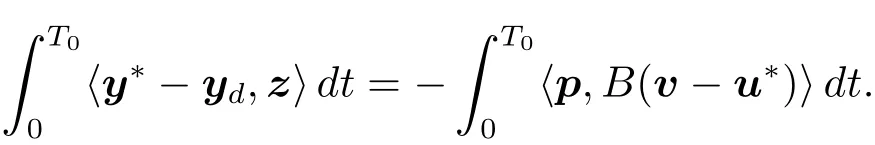
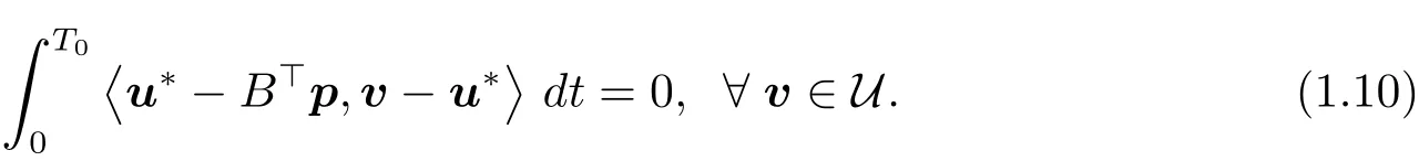
This,together with(1.8),implies that
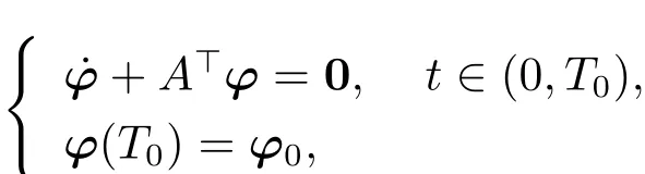
Let ?(·;T0,?0)be the unique solution to the following system
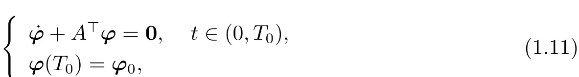
where ?0=(?01,?02,···,?0n)>.Define
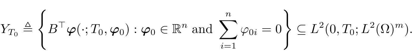
It is obvious that YT0is closed.We now claim that

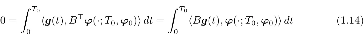
Otherwise,we would have that u??B>p∈L2(0,T0;Rm)YT0.This implies that

where g ∈ L2(0,T0;Rm).Especially,choosing f==0 in(1.13),we have that
On one hand,let w(·)be the solution to the following system
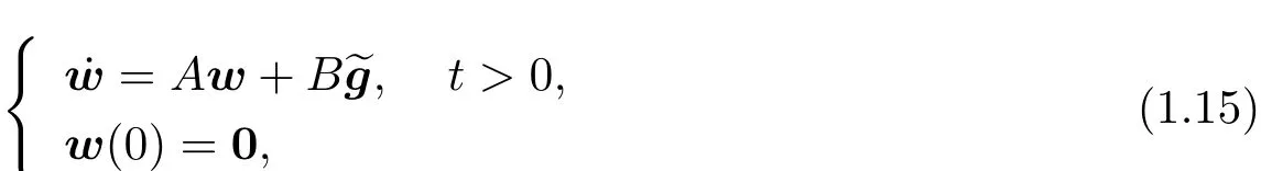
whereeg is the zero extension of g over(0,+∞).Multiplying the first equation of(1.15)by ?(·;T0,?0)and integrating it over(0,T0),by(1.11)and(1.15),we obtain that
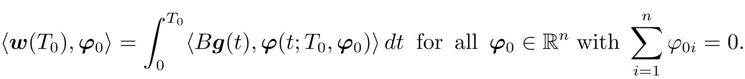
This,together with(1.14),implies that

where w(T0)=(w1(T0),w2(T0),···,wn(T0))>.
On the other hand,by(1.3),we denoteμ and α(1,1,···,1)>.Then we can directly check that

Since w(t)=eA(t?T0)w(T0)for all t≥ T0,it follows from(1.16)and(1.17)that

This implies thateg+u?∈U.By(1.10),we get that
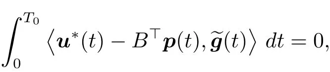
which leads to a contraction with(1.13).Hence,(1.12)follows,i.e.,there exists a q0==0,so that

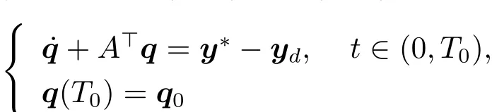
Set q(·),p(·)+ ?(·;T0,q0).Then by(1.9)and(1.18),we have that

and u?(t)=B>q(t)a.e.t∈ (0,T0).
Thus,we finish the proof of the necessity.
We next turn to the proof of“sufficiency” part.For any u ∈ U,we denote

where z(·),(z1(·),z2(·),···,zn(·)).We can easily check that(
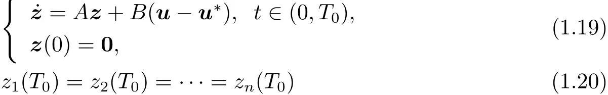
and
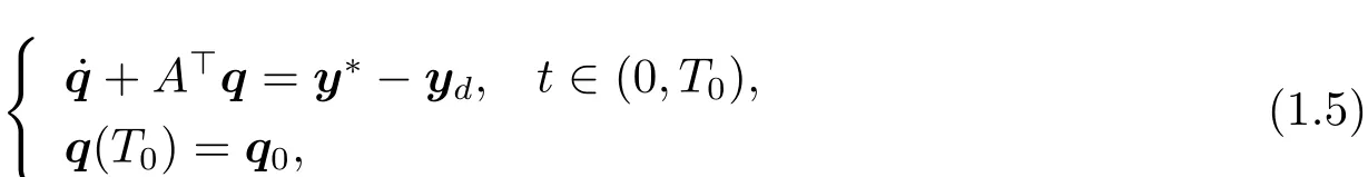
Multiplying the first equation of(1.5)by z and integrating it over(0,T0),by(1.19),(1.4)and(1.5),we obtain that
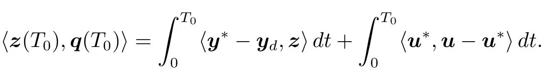
This,along with(1.20)and(1.21),implies that
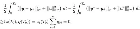
which indicates that u?is the optimal control to problem(P).
(ii)By the same arguments as those in[16],under hypothesis(H2),we observe that
We start with the proof of“Necessity” part.Let p and ?(·;T0,?0)(where ?0∈ Rn)be the unique solution to the equations
and
respectively.Define

It is obvious that YT0is closed.By similar arguments as those to prove(1.12),we have that u??B>p∈YT0,i.e.,there exists a q0∈Rn,so that

Set q(·),p(·)+ ?(·;T0,q0).Then by(1.22)and(1.23),we have that
and u?(t)=B>q(t)a.e.t∈ (0,T0).
Thus,we finish the proof of the necessity.
We next turn to the prove of“sufficiency” part.Its proof is similar to that of“Sufficiency”part in(i).We omit it here.
3 Numerical Tests
In this section,we carry out two numerical tests.The tests concern the two cases considered in Theorem 1.1,where(H1)is satisfied in Test 1 and(H2)is satisfied in Test 2.
Test 1For the framework of(i)in Theorem 1.1,we observe that the optimal control u?and the optimal trajectory y?are the solutions to following equations where y(T0)=(y1(T0),y2(T0),···,yn(T0))>,q(T0)=(q1(T0),q2(T0),···,qn(T0))>,y0,ydand T0are given,A and B will be chosen to satisfy(H1).
Let(tl)l=0,1,···,Nbe an equidistant partition of[0,T0]with the time step ?t=,i.e.,

For l=0,1,···,N,i=1,2,···,n,we set

The discretization of(3.1)gives the following system by an implicit finite dif f erence scheme
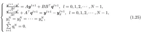
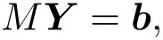
This can be reformulated as a linear system of(2N+1)×n equations MY=b,here
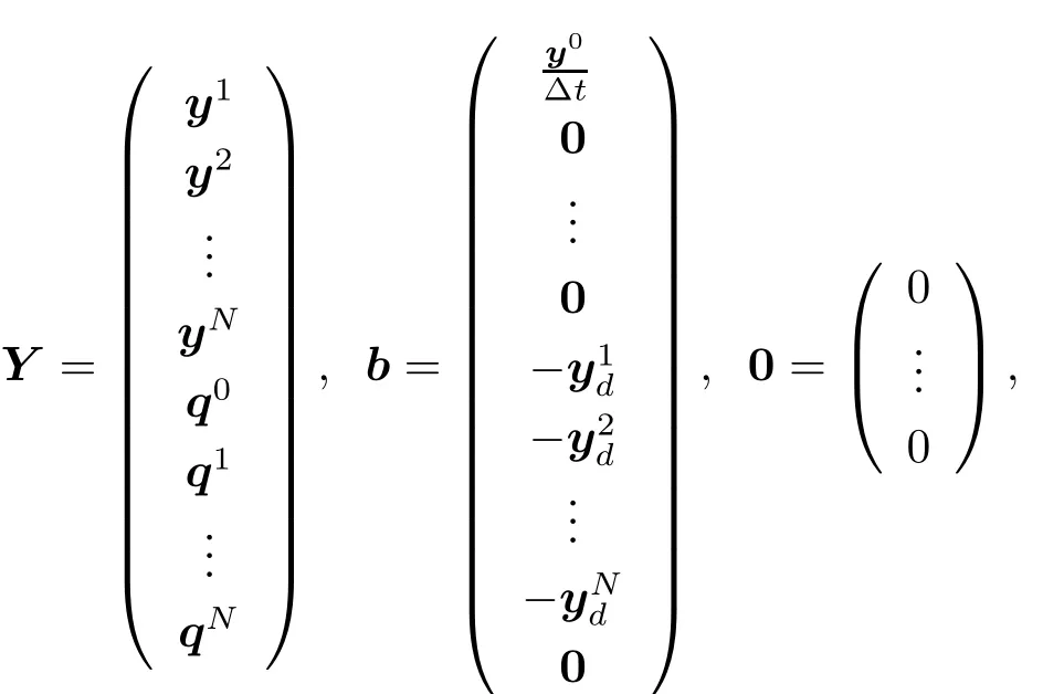
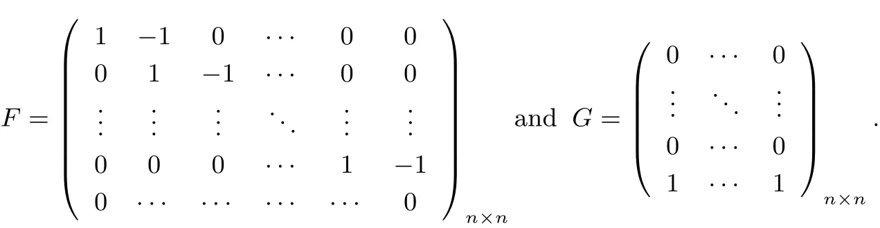
and M is a(2N+1)n×(2N+1)n matrix given by
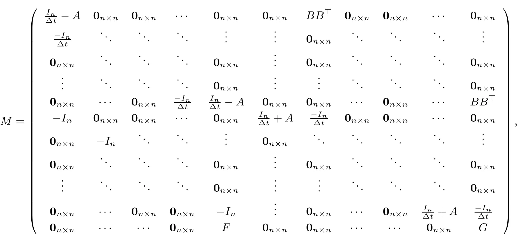
where Inis the n-dimension identity matrix,0n×nis the n-dimension zeros matrix,
Finally,we can solve(3.2)for dif f erent choice of N to obtain the numerical solution y?,then compare them with the exact solution of y?to check the convergence of the algorithm.
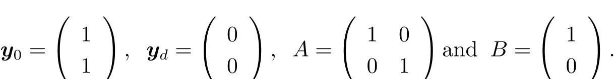
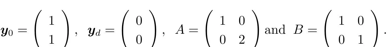
We carry out the test with n=2,m=1,T0=1,
Clearly A,B satisfy(H1),and the exact solutioncan be obtained by direct computation
Taking N=10,20,40,we can illustrate the numerical solution y?and the exact solution of y?in the following figures
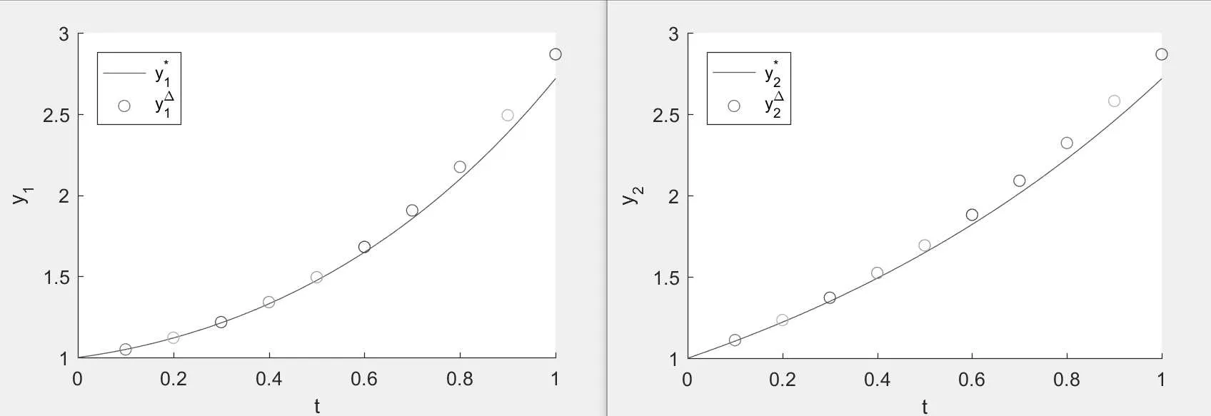
Figure 1:the empty circle is the numerical solution y?=,and the solid line is the exact solution y?=when N=10.
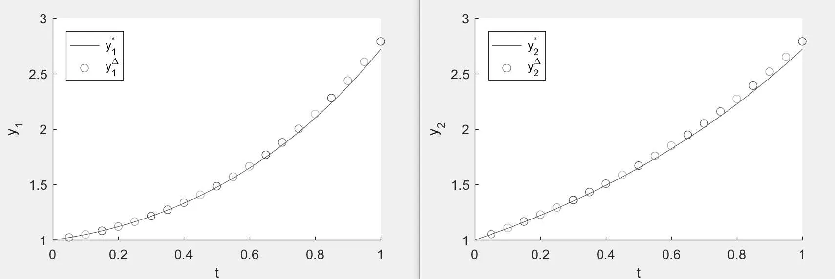
Figure 2:the empty circle is the numerical solution y?=,and the solid line is the exact solution y?=when N=20.
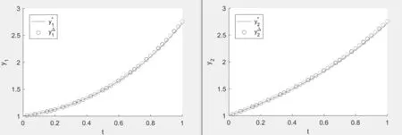
Figure 3:the empty circle is the numerical solution y?=,and the solid line is the exact solution y?=>when N=40.
Test 2For the framework of(ii)in Theorem 1.1,we see that the optimal control u?and optimal trajectory y?are the solutions to following equations
where y(T0)=(y1(T0),y2(T0),···,yn(T0))>,ydand T0are given,A and B will be chosen to satisfy(H2).
Analogously we take the same scheme as in Test 1 to obtain the discretization of(3.3)as the following system
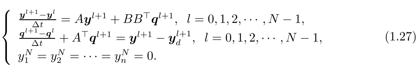
This can be reformulated as a linear system of(2N+1)×n equations:
Here

and M is a(2N+1)n×(2N+1)n matrix given by
where Inis the n-dimension identity matrix,and 0n×nis the n-dimension zeros matrix.
Finally,we can solve(3.4)for dif f erent choice of N to obtain the numerical solution y?,then compare them with the exact solution of y?to check the convergence of the algorithm.We carry out the test with n=m=2,T0=1,
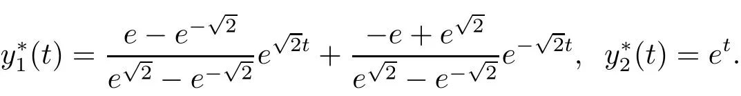
Clearly A,B satisfy(H2),and the exact solution y?=(y?1,y?2)>can be obtained by direct computation:

Taking N=10,20,40,we can illustrate the numerical solution y?and the exact solution of y?in the following figures:
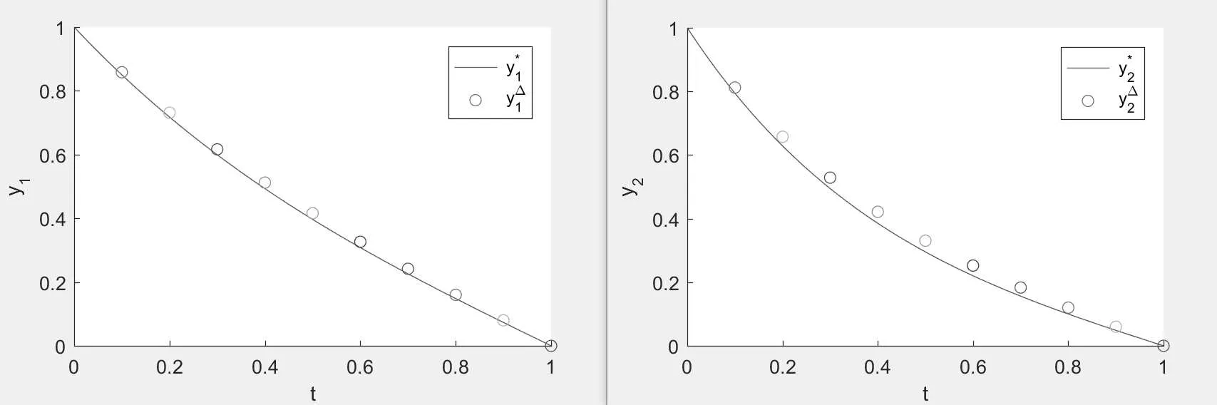
Figure 4:the empty circle is the numerical solution y?=,and the solid line is the exact solution y?=when N=10.

Figure 5:the empty circle is the numerical solution y?=>,and the solid line is the exact solution y?=when N=20.
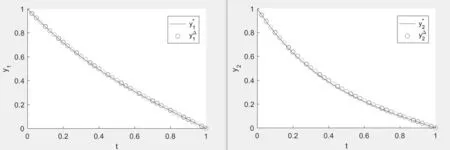
Figure 6:the empty circle is the numerical solution y?=(y?1,y?2)>,and the solid line is the exact solution y?=when N=40.
From these figures,we observe that the error between the numerical solution and the exact solution decreases with the increase of N.So,if we take the value of N large enough,the exact solution can be approximated nicely by this method.