Convergence Rates for Elliptic Homogenization Problems in Two-dimensional Domain

(College of Science,Zhongyuan University of Technology,Zhengzhou 450007,China)

§1.Introduction

This paper concerns with the asymptotic behavior of the solution for second order elliptic operators in two-dimensional domain,arising in the theory of homogenization,with highly oscillating periodic coefficients.More precisely,given a boundedC1,1domain ??R2,we consider

Throughout this paper,the summation convention is used.We assume that the matrixA(y)=(aij(y))with 1≤i,j≤2 is real symmetric and satisfies the ellipticity condition

whereλ＞0 and the periodicity condition

We also impose the smoothness condition

The convergence of the solutions is one of the main problems in homogenization theory.There are many papers about convergence rates for elliptic homogenization problems.Assume that all of functions are smooth enough,theO(ε)error estimate inL∞was presented by Bensoussan,Lions and Papanicolaou[5].In 1987,Avelcaneda and Lin[2]provedLpconvergence for solutions through the method of maximum principle.In the same year,they[3]obtainedL∞error estimate whenfis less regular than Bensoussan,Lions and Papanicolaou’s[5].Griso[7-8]obtained interior error estimates by using the periodic unfolding method.In 2010,Kenig,Lin and Shen[13]studied rates of convergence of solutions inL2andin Lipschitz domains with Dirichlet or Neumann boundary conditions.

The main purpose of this work is to study the rates of convergence of solutions in a bounded two-dimensionalC1,1domain with Dirichlet or Neumann problems.In 2014,Kenig,Lin and Shen had studied the asymptotic behavior of the Green and Neumann functions obtaining some error estimates for solutions when the dimension is greater than two.In their paper,it is much harder to find the representation formula satisfied by the oscillatory solution and homogenized solution(Proposition 2.2 in[14]).In our case,we use an extension of the ”mixed formulation”approach obtaining a very explicit representation formula foruεandu0(see(2.8))by means of the particularity of the solutions for equations in two-dimensional case.This makes the estimate becomes more simple.It is also the technical difference compared with Kenig,Lin and Shen’s[14]work.But this approach is not valid when the dimension is greater than two,the main reason is that the existence of the solution for equation(2.6)is guaranteed only in the two-dimensional case.

To the best of our knowledge,this work seems to be obtaining the optimal estimation in theL∞norm(see Theorem 3.5,Theorem 4.11).In 2003,Choe,Kong and Lee[6]studied the convergence rates for second elliptic equation with rapidly oscillating periodic coefficients in R2.They obtained‖uε?u0‖L∞(?)≤Cε‖f‖Lq(?),whereq＞2.This can be obtained via the growth estimate of Green functions.In the present paper,we derive the better growth rate of Green functions(see Theorem 3.4)and get error estimates in theL∞norm whenfis less regular than Choe,Kong and Lee’s[6].

One may consult several outstanding sources[5,12,4,10,9,1,16]for background and overview of the homogenization theory.

§2.Extension of the “Mixed Formulation”

In order to establish a very explicit representation formula foruεandu0,in this section,we use an extension of the”mixed formulation” approach.This method was originally proposed in[5].In 1997,Moskow and Vogelius[17-18]applied this method to study homogenized eigenvalues problems with Dirichlet or Neumann boundary conditions.

For a fixedf∈L2(?),letuεbe the solution of the following Poisson equation

We write this second order equation as a first order system

and proceed to look for a formal expansion of the form

whereui(x,y)andvi(x,y)are periodic in the ”fast” variabley=x/ε.

We introduce the notation▽for the full gradient andandfor derivatives in thefirst and second variables respectively.After formally identifying powers of,we obtain the following equations,

It follows from(2.1)that

In view of(2.2)and(2.3),we obtain

where functionχ(y)=(χj(y))is the solution of the following cell problem,

for each 1≤j≤2,whereY=[0,1)22/Z2.

It follows from(2.3)and(2.4)that

whereL0is a constant coefficient operator which is also called homogenized operator.The constant matrix is given by

Next definev0by

This definition make sure that(2.2)and(2.3)are satisfied.If we define periodic functionρ(y)such that

The last identity we used the fact that▽x·v1(x,y)=0.

Hence,

From the definition ofψε(x),we obtain|ψε(x)|≤Cε|▽2u0(x)|a.e.x∈?.

§3.Convergence Rates with Dirichlet Problems

The goal of this section is to establish convergence rates of solutions for the following elliptic equation Dirichlet problem,

Throughout the rest of this paper,we set

for somex0is the open ball of radiusrcentered atx0andr0is a constant.

LetGε(x,y)denote the Green functions for operatorsLεin a bounded domain ?.It follows from[3]that if ? is a boundedC1,γdomain for some 0＜γ≤1,then for anyx,y∈?,

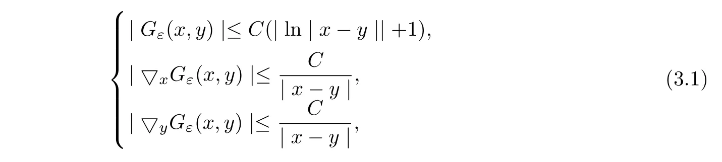
where constantCdepends only onλ,Λ,αand ?.

3.1 Convergence Rates in Lp

In order to obtain the rates of convergence inLpfor solutions,firstly,we shall establish anL∞error estimate for local solutions.Then we obtain the growth rate of Green functions.By the Green function representation of solution,we obtain convergence estimates for‖uε?u0‖Lp(?)for any 1＜p≤∞.

Lemma 3.1Suppose thatuεsatisfies

Then

whereq＞2 andCdepends onq,α,λ,Λ and ?.

ProofThe estimate follows from the maximum principle and De Giorgi-Nash estimate(Theorem 8.25 in[11]).

whereq＞2 and we have used H?lder′s inequality‖▽y(x,y)‖Lq/(q?1)(D2)≤C.This together with(3.5),completes the proof.

Lemma 3.3Assume thatuεandu0satisfy the same condition as in Lemma 3.2.Suppose that

whereq＞2 andCdepends only on Λ,q,α,λand ?.

ProofThe proof is the same as that of Lemma 3.2.Consider

where

In view of maximum principle,we obtain

It follows from(3.22)and(3.111)that

In view of(2.7)and(3.3),we have

whereGε(x,y)denotes the Green functions for operatorsLεin ?.It follows from(3.1)and H?lder′s inequality,we obtain

for anyq＞2.

This together with(3.9)gives

Then(3.5)follows from the following inequality and Sobolev imbedding Theorem[11],

This completes the proof.

Now,we obtain the growth rate of Green functions from the following theorem.

Theorem 3.4Assume thatGε(x,y)andG0(x,y)denote the Green functions for operatorsLε,L0in ? respectively.Letf∈L2(?).Suppose that

Then for anyx,y∈?,

whereCdepends onα,Λ,λand ?.

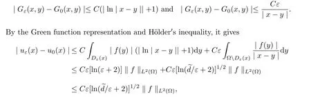
ProofFirstly,we fixx0,y0∈? and letr=|x0?y0|/4.Let(Dr(y0)).From the Green function representation,we have

It follows from(3.5)and(3.11)that

whereq＞2.

SinceLε(Gε(x0,y))=L0(G0(x0,y))=0 inDr(y0)andGε(x0,y)=G0(x0,y)=0 on Γr(y0),we invoke Lemma 3.2 to conclude that

where we have used(3.1).This completes the proof.

As an application of Theorem 3.4,we obtain convergence estimates of‖uε?u0‖Lp(?)for any 1＜p≤∞.

Theorem 3.5Assume thatuε∈H1(?)and for givenf∈Lq(?).Suppose thatuεis the solution of Dirichlet problems

Then these estimates

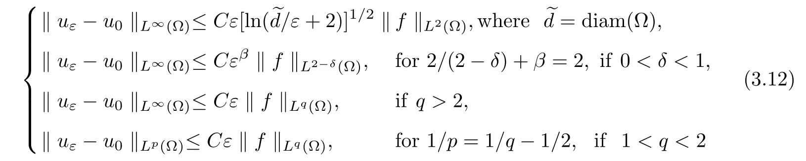
hold,whereCdepends onq,α,Λ,λand ?.

ProofIn view of(3.1)and(3.10),we obtain convergence rates for Green functions

where 2/(2?δ)+β=2 and 0＜δ＜1.

The third estimate follows from H?lder′s inequality directly.

The last inequality follows from(3.10)and Hardy-Littlewood-Sobolev theorem of fractional integration(Chapter 5,Theorem 1 in)[19].This completes the proof.

3.2 Gradient Error Estimates

In order to get the Lipschitz convergence rate estimate for solutions,we introduce a boundary correction functionθε∈H1(?),defined by

whereGε(x,y)denotes the Green functions for operatorsLεin ?.This gives

where we have also used theC2,αestimate‖u0‖C2,α(?)≤C‖f‖C0,α(?).This completes the proof.

§4.Convergence Rates with Neumann Problems

In this section,we shall consider the following Neumann problems,

where

denotes the conormal derivative withLεandn=(n1,n2)denotes the outward unit normal to??.

Without loss of generality,we also assume the compatibility condition

LetNε(x,y)denote the Neumann functions for operatorsLεin a boundedC1,1domain ?.It follows from[15]that if ? is a boundedC1,γdomain for some 0＜γ≤1,then for anyx,y∈? andβ＞0,

where constantCdepends onα,λ,Λ and ?.

Remark 4.1These estimates for Neumann functions inare not optimal in the literatures,at least we can not find a reference.One should expect the logarithmic estimate,but the best estimates the author find are that in[15].

4.1 Convergence Rates in Lp

Following the same line of research about convergence rates inLpfor solutions with Dirichlet boundary conditions,although a bit more complicated,this subsection is devoted to the case of Neumann boundary conditions.Firstly,we establish the conormal derivative associated withLε.

This completes the proof.

Lemma 4.3Suppose thatuεsatisfies

Then

whereq＞2 andCdepends onq,λ,Λ,αand ?.

ProofThis estimate had been proved by Kenig,Lin and Shen(Theorem 3.1 in[15]).

Next,we obtain anL∞estimate for local solutions.

Lemma 4.4Assume thatuε∈H1(D4r)andu0∈W2,q(D4r)for some 2＜q≤∞.Suppose that

Then,for anyβ∈(0,α),

whereCdepends only on Λ,q,α,λand ?.

ProofBy scaling we may assume thatr=1.Let

In view of(2.8)and Lemma 4.2,we obtain

This implies that

Finally to estimate,it follows from Lemma 4.3 that

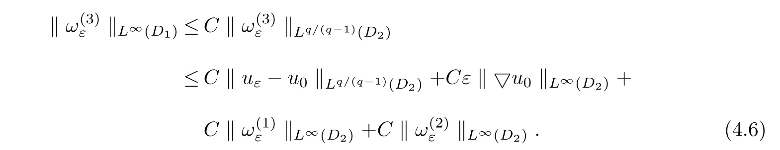
This together with(4.4)and(4.5),gives(4.2).

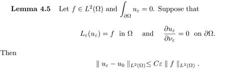
ProofThis estimate follows from(Corollary 5.3 in)[13]and the following inequality,

This completes the proof.

Theorem 4.6Assume thatNε(x,y)andN0(x,y)denote the Neumann functions for operatorsLε,Loin ? respectively.Then for anyx,y∈? andβ∈(0,α),

whereCdepends onα,Λ,λ,βand ?.

ProofThis estimate follows from(4.1),Lemma 4.4 and Lemma 4.5.The proof is the same as that of Theorem 3.4.

As an application of Theorem 4.6,we obtain error estimates of‖uε?u0‖Lp(?).

ProofIn view of(4.1)and(4.7),we obtain convergence rates for Neumann functions,

for anyβ∈(0,α).

By the Neumann function representation and H?lder′s inequality,it gives

which gets the first estimate.

The rest of the proof is the same as that of Theorem 3.5.

4.2 Gradient Error Estimates

In this subsection,we will establish gradient error estimates of solutions for Neumann problems.This can be obtained via uniform regularity estimate,which is an important tool in the study of convergence problems for solutions.In order to deal with boundary term,we introduce a boundary correction functionξε∈H1(?),defined by

Let

In view of(2.8)and Lemma 4.2,we obtain

Lemma 4.8Suppose that matrixAsatisfies(1.1)～(1.3).Let ? be a boundedC1,1domain andF∈Lp(?)for any 1＜p＜∞.Then the weak solution to

satisfies the estimate

whereCdepends only onλ,p,Λ,αand ?.

ProofThis estimate had been proved by Kenig,Lin and Shen(Lemma 4.2 in[15]).

Then the estimate

holds,whereξεdenotes the boundary correction function forLεin ?.

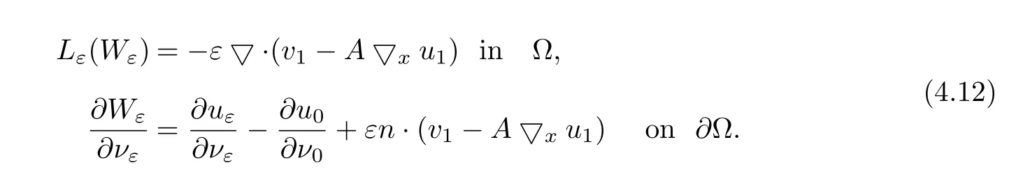
ProofIt follows from(4.11)and(4.12)that

Since

we invoke Lemma 4.8 to obtain(4.13).This completes the proof.

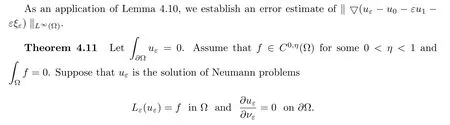
Lemma 4.10Suppose that ? is a boundedC1,1domain and matrix A satisfies(1.1)～(1.3).Letuεbe a solution of the Neumann problems

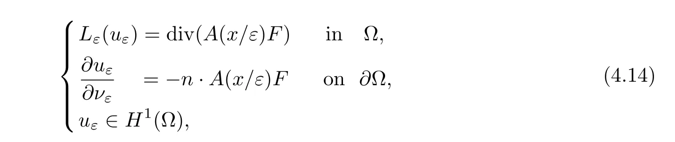
whereF∈C0,η(?)for some 0＜η＜1.Then▽uε∈L∞(?)and

whereCdepends only onλ,Λ,ηand ?.

ProofIn view of(4.14)and the Neumann function representation,we obtain

It follows that for anyx∈?,

Note that ifFj(x)=?δjk,thenuε(x)=xkis a solution of(4.14).It follows from(4.15)that

In view of(4.15)and(4.16),we obtain

Hence,

This completes the proof.

Then the estimate

is valid,whereCdepends only onλ,η,Λ and ?.

ProofIn view of(4.11)～(4.12)and Lemma 4.10,we obtain

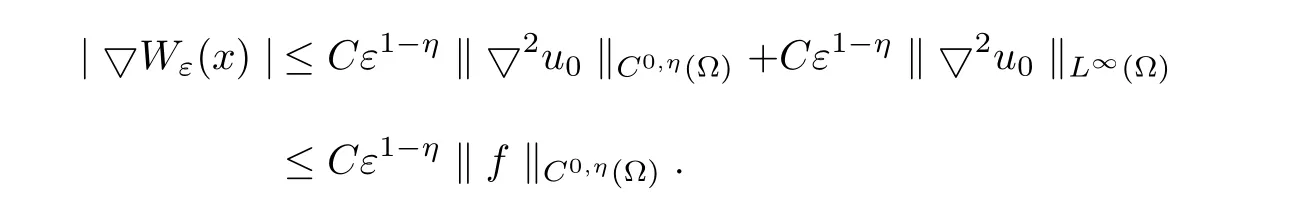
This completes the proof.

[1]ALLAIRE G.Shape Optimization by the Homogenization Method[M].New York:Springer-Verlag,2002.

[2]AVELLANEDA M,LIN Fang-hua.Homogenization of elliptic problem withLpboundary data[J].Appl Math Optimization,1987,15(1):93-107.

[3]AVELLANEDA M,LIN Fang-hua.Compactness methods in the theory of homogenization[J].Comm Pure Appl Math,1987,40(6):803-847.

[4]BRAICLES A,DEFRANCESCHI A.Homogenization of Multiple Integrals[M].Clarenoon:Oxford,1998.

[5]BENSOUSSAN A,LIONS JL,PAPANICOLAOU G.Asymptotic Analysis for Periodic Structures[M].North-Holland:Amsterdam,1978.

[6]CHAO HJ,KONG KB,LEE CO.Convergence inLpspace for the homogenization problems of elliptic and parabolic equations in the plane[J].J Math Anal Appl,2003,287(2):321-336.

[7]GRISO G.Error estimate and unfolding for periodic homogenization[J].Asymptot Anal,2004,40(3-4):269-286.

[8]GRISO G.Interior error estimate for periodic homogenization[J].Anal Appl,2006,4(1):61-79.

[9]GIORANESCU D,DONATO P.An Introduction to Homogenization[M].Clarenoon:Oxford,1999.

[10]GIORANESCU D,SAINT J,PAULIN J.Homogenization of Reticulated Structures[M].New York:Springer-Verlag,1999.

[11]GILBARG D,TRUDINGER NS.Elliptic Partial Differential Equations of Second Order[M].New York:Springer-Verlag,1998.

[12]HORNUNG U.Homogenization and Porous Media[M].New York:Springer-Verlag,1997.

[13]KENIG CE,LIN Fang-hua,SHEN Zhong-wei.Convergence rates inL2for elliptic homogenization problems[J].Arch Rational Mech Anal,2012,203(3):1009-1036.

[14]KENIG CE,LIN Fang-hua,SHEN Zhong-wei.Periodic homogenization of Green and Neumann functions[J].Comm Pure Appl Math,2014,67(8):1219-1262.

[15]KENIG CE,LIN Fang-hua,SHEN Zhong-wei.Homogenization of elliptic systems with Neumann boundary conditions[J].J Amer Math Soc,2013,26(4):901-937.

[16]MANECITCH LI,ANDRIANOV IV,OSHMYAN VG.Mechanics of Periodically Heterogeneous Structures[M].New York:Springer-Verlag,2002.

[17]SANTOSA F,VOGELIUS M.First-order Corrections to the Homogenized Eigenvalues of a Periodic Composite Medium[J].SIAM J Applied Math,1993,53(6):1636-1668.

[18]MOSKOW S,VOGELIUS M.First-order corrections to the homogenised eigenvalues of a periodic composite medium.A convergence proof[J].Proc Roy Soc Edinburgh,1997,127(6):1263-1299.

[19]STEIN EM.Singular Integrals and Differentiability Properties of Functions[M].New Jersey:Princeton University,1970.