
The Reliability of Global and Hemispheric Surface Temperature Records
2016-11-25 03:10:12PhilipJONES
Advances in Atmospheric Sciences 2016年3期
Philip JONES
1Climatic Research Unit,School of Environmental Sciences,University of East Anglia,Norwich NR4 7TJ,UK
2Center of Excellence for Climate Change Research,Department of Meteorology,King Abdulaziz University,Jeddah,Saudi Arabia
(Received 31 August 2015;Revised 22 October 2015;Accepted 9 November 2015)
The Reliability of Global and Hemispheric Surface Temperature Records
Philip JONES?1,2
1Climatic Research Unit,School of Environmental Sciences,University of East Anglia,Norwich NR4 7TJ,UK
2Center of Excellence for Climate Change Research,Department of Meteorology,King Abdulaziz University,Jeddah,Saudi Arabia
(Received 31 August 2015;Revised 22 October 2015;Accepted 9 November 2015)
The purpose of this review article is to discuss the development and associated estimation of uncertainties in the global and hemispheric surface temperature records.The review begins by detailing the groups that produce surface temperature datasets.After discussing the reasons for similarities and differences between the various products,the main issues that must be addressed when deriving accurate estimates,particularly for hemispheric and global averages,are then considered. These issues are discussed in the order of their importance for temperature records at these spatial scales:biases in SST data, particularly before the 1940s;the exposure of land-based thermometers before the development of louvred screens in the late 19th century;and urbanization effects in some regions in recent decades.The homogeneity of land-based records is also discussed;however,at these large scales it is relatively unimportant.The article concludes by illustrating hemispheric and global temperature records from the four groups that produce series in near-real time.
surface temperature data,SST,temperature homogeneity,temperature biases,urbanization
1.Introduction
A number of groups routinely update gridded datasets of surface temperature for land and marine regions,which can beusedtoproducetimeseriesofglobaland hemispheric temperatures.The four main groups are:the UK Meteorological Office Hadley Centre/Climatic Research Unit,which produces HadCRUT4(Morice et al.,2012;http://www.cru.uea. ac.uk/cru/data/temperature/,andhttp://hadobs.metoffice.com/ hadcrut4/)—an updated version of HadCRUT3(Brohan et al.,2006);the US National Centers for Environmental Information(NCEI;Karl et al.,2015;https://www.ncdc.noaa.gov/ climate-monitoring),which is an updated version of Smith et al.(2008)and Vose et al.(2012);the Goddard Institute for Space Studies(GISS;Hansen et al.,2010;http://data.giss. nasa.gov/gistemp/),which is an updated version of Hansen et al.(1999,2006);and the Berkeley Earth Group(BEST;Rohdeetal.,2013a,2013b;http://berkeleyearth.org/).Oneother group monitors land-based temperatures(Lugina et al.,2006) andanothermonitorsSST(Ishiietal.,2005).Surfacetemperature datasets are comprised of measurements from the land (from air temperatures at fixed locations)and SST data from the ocean(from moving ships and buoys).SST data are used fortheoceansinsteadofmarineairtemperatures(MAT,taken by ships),as a few SSTs in an area of ocean are much morereliable than the same number of MAT measurements.Additionally,the number of MAT measurements must be further reduced by half,due to daytime heating caused by the ship, so only night-time MAT(see discussion in Kent et al.,2013) can be used.Data from the two components are combined as anomalies from a base period.The base period,however, is different for the four data sets:1961–90 for HadCRUT4; 1901–2000 for NCEI;and 1951–80 for GISS and BEST.
All the groups use much the same input data,but employ different approaches to interpolation to develop gridded products.HadCRUT4 and NCEI both use a 5?×5?latitudelongitude grid that is produced first for separate domains for land and ocean.These two gridded products have overlaps at coastlines and islands and are combined in different ways by the four groups.HadCRUT4 combines land data from CRUTEM4(Jones et al.,2012)with SST data from HadSST3 (Kennedy et al.,2011a,2011b;see also Kennedy,2014). NCEI use land data from the ISTI database(Rennie et al., 2014)and their ERSSTv4 dataset of SST anomalies over the ocean(Huang et al.,2015;Liu et al.,2015).GISS data are derived by first averaging all the land station data(from NCEI) into 160 approximately equal-area boxes,and then combining these with SST values(currently using ERSSTv4)from marine areas.BEST uses numerous station datasets from NCEI,and also those used by CRUTEM4 combined with marine data from HadSST3.
If there are no data for a given month in one of the grid boxes,theHadCRUT4valueismissing.Alltheotherdatasetsperform some sort of spatial infilling to produce more globally complete fields–NCEI by using an eigenvector-based technique,where this is judged to produce statistically reliable estimates;GISS uses 160 equal-area boxes effectively to provide some infilling in data-sparse areas,so only a few of the boxes are completely missing for all months;and BEST use kriging procedures(see Rohde et al.,2013a,2013b).The amount of infilling undertaken with NCEI,GISS and BEST is unknown without station coverage for each month/year. Maps of all stations used are unhelpful without knowing their data availability,especially before the 1950s.Additionally,a fifth group,the Japanese Meteorological Agency,combines the Ishii et al.(2005)SST data with land stations from NCEI, http://ds.data.jma.go.jp/tcc/tcc/products/gwp/temp/ann wld. html,but the method has not been formally published.Despite these differences in the methods used to combine the basic data,the hemispheric-and global-scale time series are very similar[see the trends calculated over three different periods in Table 3.3 of Trenberth et al.(2007)for IPCC AR4, and Table 2.7 of Hartmann et al.(2013)for IPCC AR5].In section 7 of the present paper,trends for global averages over three periods(1901–2014,1951–2014 and 1979–2014)are calculated.
?The author 2016
The purpose of this article is to first discuss(in section 2) theprincipalreasonsforthesimilaritiesatlargespatialscales, and then(in section 3)the important issues that need to be considered to ensure reliability and to assess the accuracy of the monthly and annual estimates(for hemispheric and global averages and also at the grid-box scale).Section 4 illustrates these for the biases(SSTs,exposure and urbanization),while land-station homogeneity is addressed in section 5.Section 6 discusses the results from a number of reanalyses of the climate system(e.g.,ERA-Interim;Dee et al.,2011)in the context of changes in spatial coverage through time.With all this knowledge,section 7 discusses the hemispheric and global analyses produced by the four groups,and section 8 concludes.
2.Similarity and homogeneity of large areaaverage time series
There are three principal reasons for the close similarity between the four independently derived data series.The first isthattheyusemuchthesameraw(monthly-mean)inputdata for the land areas and separately similar input data(International Comprehensive Ocean Atmosphere Dataset,ICOADS) for the marine areas.The second is that similar bias and homogeneity adjustments are applied to both sets of data,particularly for the ocean,and these form the main discussion points of this paper.While there are some minor differences in the input data and the adjustments applied,many of the homogeneity issues are essentially random;so,when averaged over large areas,the differences tend to cancel out.The third factor is often ignored and poorly understood;namely, that grid-box temperature time series from neighbouring locations are highly spatially correlated.Thus,even though there are records from thousands of sites on land and from millions of measurements from ships and buoys across the world’s oceans,the“effective”number is much less than this.Estimates(using both observational data and globally complete climate model data)indicate that the effective number of independent observations at the monthly timescale for the global surface area is about 100(see Jones et al.,1997). Thus,provided input datasets have at least 100 well-spaced sampling points for which the data are relatively free of nonclimatic biases,even if the locations of these sites are different between the different groups,they will lead to very similar large-scale area averages.For annual or decadal averages the required number of well-spaced locations can be substantially less than 100.
A similar situation exists for pressure data.Here,the correlation decay length is similar to that for temperature,so relatively few sites can produce reliable area averages.For precipitation,however,the required number of data series to produce reliable area averages is much greater than for temperature,as correlation decay lengths are much smaller.The number of locations required to derive similar datasets from daily temperature averages would be larger,as at the daily timescale correlation decay lengths would also be smaller.
The relatively small number of locations required to estimate large-scale area averages accurately means that,even for early parts of the temperature record when the data network was relatively sparse,area averages are reliable back to the second half of the 19th century.A test of the adequacy of the evolving network of temperature data sites for deriving large area-average time series is provided by Le Treut et al. (2007,Fig.1.3).Here,many of the series developed before 1985(all of which are just for the land regions of the world) are compared and shown to agree well.Even the record developed by K¨oppen(1873)for the Northern Hemisphere land masses is similar to averages developed today by CRUTEM4. The adequacy of the network used by Callendar(1938,1961) is also excellent when compared to CRUTEM4(Hawkins and Jones,2013).
The adequacy of early networks has also been illustrated using subsamples involving the use of present-day regions that had good sampling in the 19th century.Parker et al. (2009),for example,have shown that the number of sites required to produce a reliable area average is small(see their Fig.1).They did this by calculating global land averages using a limited set of 5?grid boxes,and then with another analysis offset from the first by 10?of longitude and latitude. Earlier,Jones(1994)used a sparse but more constant network of stations to show that the sparser networks available in the second half of the 19th century could reproduce the global average reliably on decadal timescales and so ensure the consistency of large-scale area-average time series.Individual months and years may differ,particularly prior to 1900,but sparse networks are very reliable for decadal and longer-timescale averages.
Network adequacy has also been discussed by Cowtan and Way(2014),who claim that HadCRUT4 underestimates warming in the last 15 years due to missing grid boxes inthe Arctic.Cowtan and Way(2014)infill all missing grid boxes in HadCRUT4 from 1979 onwards using reanalysis products,lower tropospheric temperatures,or by kriging—not just across the Arctic,but also for the Antarctic,parts of Africa,and a few smaller areas.Using reanalysis can cause problems in the Antarctic(Jones and Lister,2015)and is not to be recommended.Infilling by kriging tends to produce fields that are smoother than observed data show.In section 7,it is shown that the trends of the various datasets demonstrate that warming rates in HadCRUT4 are not significantly different from the other three datasets(see Table 1).
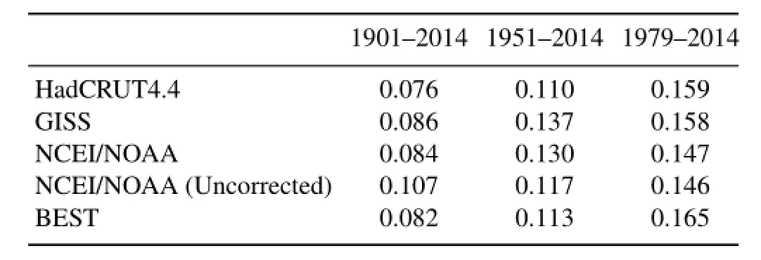
Table 1.Temperature change[?C(10 yr)-1]explained by the linear trend for the global annual average of the four datasets introduced in section 1 of this paper.These series are plotted in the lower panel of Fig.1.All trends for all three periods are statistically significant at the 99%confidence level,or better.
The strong spatial correlation of temperature is also important in paleo-temperature reconstructions from proxy data.Here,the number of sites is much fewer than for instrumental data,but reliable area averages can still be produced (see Jansen et al.,2007).Further back in time,millennial-and multi-millennial-scale temperature histories are derived from a few ice cores and/or deep sea cores(see Masson-Delmotte et al.,2013).
3.Issues to consider in series adjustment and error assessment
The effective number of spatial degrees of freedom is one of the key parameters in estimating the statistical uncertainty in estimates of large-scale averages.In an earlier study by the HadCRUT group(Brohan et al.,2006),estimated uncertainties also account for uncertainties in homogeneity and bias adjustments to the basic data,possible urbanization influences,as well as the effects of sparser sampling in the earlier years.The incorporation of these components is complicated by the fact that some issues cancel by the number of measurements(particularly those due to land-station homogeneity), while the biases tend to be consistent so do not cancel.In order for uncertainty errors to be widely used,Morice et al. (2012)introduced the concept of multiple,but equally plausible,realizations of the past.The HadCRUT4 dataset has developed 100 such realizations with a best guess,the median value for each grid box,and the median of the 100 realizations of global and hemispheric averages.The range of these realizations expands for years earlier in the record,but is still quite low in regions with good coverage back to 1850. Smith and Reynolds(2005)have also looked at the effects of sparser coverage in earlier years.
Knowledge of the potential sources of error and their correlative structure is key information if the uncertainties in the global temperature record are to be reduced.The greatest potential for improvement will come from infilling data gaps in early years,particularly through the incorporation of more marine data[where improvements in metadata will also be important–as evidenced in the work of Thompson et al. (2008,2009)].As will be shown in this paper,the greatest uncertainty is in the marine data before World War 2,and this has recently been well illustrated by Karl et al.(2015).
To discuss the different uncertainty components,it is necessary to understand their structure;but before that,there is a need to define a few terms commonly used in climatology. There are three basic issues in the development of the gridded temperature products and global and hemispheric means: homogeneity of the basic raw station or marine time series; large-scale systematic biases that might affect large areas; and the lack of coverage in parts of the world,particularly before the 1950s.These will be discussed in the next sections in their order of importance for the large-scale averages:biases,coverage,and homogeneity of the individual site series. At the local(grid-box)scale,the order of importance would differ:coverage,then homogeneity,and finally bias.The fact that the order of importance depends on the spatial scale is a particularly vital aspect to realize.Additionally,the components of the uncertainty are independent of each other,so may be combined in quadrature(Brohan et al.,2006;Morice et al.,2012),as opposed to being additive in nature.
It is important to note,however,thatthese problems apply to the original(raw)input data.For the data that are used to produce standard area-average time series,corrections have been applied to remove,as far as possible,these potential sources of error.The fact that four different organizations have made such corrections independently is a testimony to the robustness and accuracy of the resulting homogenized data(see this illustrated in section 7).Related to this,adjustments for land data are estimated completely independently from the marine series,so these two components mutually support each other.
4.Biases
Biases are homogeneity issues that affect large portions of the observational dataset.They may be smaller in magnitude than the effects of site moves and other factors(see section 5),but they can be important if they similarly affect significant fractions of the basic input data.These will be discussed in order of importance,as measured by their impact on hemispheric-and global-average series.The three most important factors are:methods of measuring SST;exposure issues with temperature recorded at land stations before the development of louvred screens;and the time-varying effects of increasing urbanization due to the growth of cities(see also Jones and Wigley,2010).This third factor is linked to the representativeness of the site in the context of possibleland-use or environmental change across the grid box within which it is located.Land station homogeneity is discussed in section 5.
4.1.SST measurements
Any issue of homogeneity or bias in measuring SSTs will have a serious impact on global temperature estimates because almost 70%of the planet’s surface is ocean.The history of marine instrumental measurements goes back to the 18th century and the basic meteorological measurements(not just SST,but air temperature,pressure,wind direction and speed,etc.)were entered into ship logbooks.Even before instruments,ships kept logbooks as these were essential for navigation.
The first SST measurements were taken using wooden buckets tied to a rope.A sample of sea water was hauled onto the ship’s deck and the temperature measured.In the earliest years these measurements came mostly from voyages of exploration.By the early 19th century a whole array of measurements,including SST became a routine part of life at sea(Maury,1855).The advent of steamships in the mid-19th century led to ships increasing their speed and deck height above the sea surface.By the late-19th century,many SST measurements were made with canvas buckets,which were more flexible and much cheaper to construct.The use of canvas buckets continued on most merchant and naval vessels up to about 1940.Bucket use continued after this,but designs were improved(see Kent et al.,2010).
When SST data were first examined in detail by climatologists in the 1970s(see references discussed by Folland and Parker,1995;Kent et al.,2010;and Kennedy,2014),it was soon realized that the method of measurement might influence the results.Between the wars there were a number of comparisons made of different measurement techniques on research vessels and on cruises,i.e.,comparisons of different types of bucket,as well as with thermometers fitted into the engine cooling-water intake pipes of ships(see Kent et al.,2010;and Kennedy,2014 for details).More comparisons were undertaken in the 1960s and 1970s,and it was at this time that an extra code was added into both logbooks and transmitted data to indicate how the measurement was made (Woodruff et al.,2011).
The different thermal properties of the buckets:wooden, canvas,and also,more recently,rubber,mean that to use these data it is necessary to determine their relative biases, and to develop a history of which types of bucket were used. Bucket-type biases have been extensively assessed by Farmer et al.(1989)and Folland and Parker(1995).Assessments are continuing as more of the history of recording is being found and more ship-logbook data digitized[see more recent discussion in Ishii et al.(2005),Kennedy et al.(2011a,2011b), Kent et al.(2013),and Kennedy(2014)].
With regard to changing instrumentation,a basic assumption is that wooden buckets dominated in the 19th century, canvas buckets from 1900 to 1941,and engine intake measurements from then on.These were not,of course,abrupt changes,but spatially variable transitions over time,so correcting for these changes is not a simple task(Kennedy, 2014).The importance of these measurement technique biases is evident from the average size of the adjustment across the world’s oceans–canvas bucket measurements need to be raised by about 0.4?C between 1900 and 1941 compared to engine intakes.The main cause here is the evaporative cooling of the sea water between the times of sampling and reading of the thermometer.The procedures provide corrections that can be applied for each part of the ocean with different values during the seasonal cycle.Temperatures measured in wooden buckets before the 1890s must also be raised relative to engine intake measurements,but by smaller amounts than for canvas buckets.Uncertainties in these adjustments are also incorporated in the overall error range accompanying each grid-box or larger-scale value[see discussion related to the multiple realizations in Kennedy et al.(2011b) and Morice et al.(2012)].These uncertainties are dependent on the size of the adjustments,so are larger for the canvas as opposed to wooden buckets.Thus,even though coverage is sparser in the late 19th century,the uncertainties are larger between 1910 than 1940 than those from the earlier sparser coverage.
Although the major issues with SST data relate to the period before about 1940,there are still issues with recording in recent times.First,recent work has suggested that SST data for the period 1945 to 1960 are too cold(Thompson et al.,2008,2009).This is related to many of the measurements in this period being taken by British naval ships,which seem to have continued their canvas bucket method of sampling. These issues are being resolved with improved metadata and by attempting to relate individual measurements to the ships that took them(see discussion in Kennedy,2014),but for about 30%of the SST observations during the period 1950–75,the measurement method is unknown.As stated earlier, buckets continued to be used after 1945,but designs were also much improved to minimize the bias(see Kent et al., 2010).Second,since the late 1970s,there have been major changes to the marine observing system,with the principal aim of improving weather forecasts and seasonal climate predictions.Satellites began to measure SSTs at this time,and fixed buoys have been deployed in the equatorial Pacific to help ENSO predictions.Further,since the late 1980s a large numberofdriftingbuoyshavebeenregularlydeployedacross the world’s oceans.Little consideration was given to the homogeneity of measurements at the time these instrumental changes and additions were made.
As a consequence,when detailed comparisons have been made,potentially important inhomogeneities have been discovered[see discussion in Kennedy(2014),Huang et al. (2015),and Liu et al.(2015)].For example,it seems that the new drifting buoys estimate SST values slightly lower than ships by 0.1?C to 0.2?C,so their use might introduce a spurious cooling in the record.More extensive discussion of the SST adjustment procedures are provided by the different data centres[see Kennedy et al.(2011a,2011b)and Kennedy (2014)for HadSST3,and Huang et al.(2015)and Liu etal.(2015)for ERSSTv4].The recent study by Karl et al. (2015)illustrates that SST adjustments are by far the largest factor impacting hemispheric and global temperature measurements.If the adjustments were not applied then centurytimescale warming would be greater,and there would be a major discrepancy between the land and marine components prior to about 1940.This will be illustrated in section 7.
4.2.Exposure of thermometers
The problem of thermometer exposure,primarily to avoid the direct impact of sunshine on the instruments,was solved during the mid-to-late 19th century with the invention of screens.The problem had been recognized for many decades. Many different variants were tried,but it wasn’t until the development of white-louvred screens by Stevenson around 1870(https://en.wikipedia.org/wiki/Stevenson screen)that consistent exposures were established.Louvred screens have had different names around the world,e.g.,“cotton region shelters”in the United States.Other changes to instrument exposure have also taken place in different regions around the world[see Parker(1994);and Trewin(2010)for extensive discussions].Prior to the development of screens,thermometers were generally positioned on north wall locations of buildings in the NH,so as not to be in direct sunlight.Despite this,they would have received some sun exposure during the early morning and late evenings during the summer, particularly the farther north the location.Before the use of screened locations,it was likely that air temperatures during the summer half of the year could be biased warm.Measurements during the winter half of the year would be unaffected.
Although the long-term homogeneity of station temperature series can be assessed(see section 5 for more discussion of this issue),the accuracy of these approaches in early years in Europe has been questioned by some authors,particularly for measurements made during the summer(see Moberg et al.,2003;Jones et al.,2003),as all series are similarly affected by screens being introduced in some regions at the same time.The discussion in these papers has centred on two aspects of long temperature series:(1)the warmth of summer temperatures in the pre-1880 period;and(2)the lower longterm warming rates in summer compared to the other three seasons.Crucially,if these issues are important,it will be regional in nature(especially in Europe and for the early parts of individual station records),but they will be of little significance for global-scale changes over the period since 1880.
Moberg et al.(2003)showed that the long-term warming in Swedish winters is consistent with changes in the atmospheric circulation(the North Atlantic Oscillation in this case)and the warming of SSTs in the North Atlantic,so is likely to be reliable.The reliability of the summer data is harder to determine,however.The circulation and local SSTs influence summer temperatures considerably less,and the principal determining factor here is the radiation received. This can be estimated from long series of cloudiness data but the long-term homogeneity of cloudiness data from early observers is beset with even more problems than for temperatures,and so cannot help to assess the reliability of long summer temperature series.
When any change to observing practice takes place,it is always recommended that parallel measurements are made [see the GCOS Monitoring Principles in Bojinski et al. (2014)].This doesn’t always happen,and even if it did in the 19th century,the comparison measurements have probably not survived.Climatologists have recently begun to collect modern parallel measurements to attempt to resolve these instrument exposure issues.Two examples of this type of work are studies in the Greater Alpine Region(GAR)by B¨ohm et al.(2010)and in Spain by Brunet et al.(2011).The former used parallel measurements at one site in Austria,which enabled the differences between the old and modern exposure methods to be estimated and related to the directional exposure of all earlier sites in the GAR.The Spanish example rebuilt screens from 19th century diagrams and made modern parallel measurements,again developing correction formulae to apply to the original 19th century data.The results were similar in both cases—summer temperatures on average were recorded about 0.4?C warmer with the old,compared to the modern,exposures.These results are very similar to pioneering assessments made at Adelaide in Australia(Nicholls et al.,1996).It is believed that instrumental series across much of Australia before 1910 are affected(Trewin,2010).
Assessment of early instrumental exposure is vital not just for long-term homogeneity,but also for the response of many natural proxies(particularly trees)to summer temperatures.Temperature reconstructions from proxy data records clearly require the primary temperature data against which the proxy data are calibrated to be reliable.If the homogeneity of pre-1900 temperature records from individual sites could be improved,this could enhance the reliability of such temperature reconstructions.
4.3.Urbanization effects
Station history information often shows that many sites began at locations in small towns,and that,over the last 100 years,some of these towns have developed into major cities. Such urban growth is likely to affect temperature records from urban sites,and warming trends from such sites are likely,on average,to be larger than if the city or town were not there(see review by Arnfield,2003).In climatology,this issue is referred to as the urbanization effect or the urban heat island.The implication of this effect for gridded datasets is that urban-affected sites will no longer be representative of the majority of the grid box.This could potentially impact large-scale temperature averages if gradually more of the sites during the 20th century are located in urban areas.The issue is not the urbanization effect per se,but whether nearby rural and urban locations show similar long-term trends.For example,city centre sites in London and Vienna are warmer than their rural counterparts,but the urban time series during the 20th century change at exactly the same rate(see Jones et al.,2008;Jones and Lister,2009).
Numerous papers have addressed urban climates and found large differences between city centre sites and rural neighboursforindividualdayandnighttemperatures(seeref-erences in Arnfield,2003)but these studies are generally not relevant to the global-scale data bases described here.This is because most of these comparisons only consider days that maximise the urban/rural difference and so are not directly relevant in the context of long-term monthly averages for typical(non-city-centre)weather stations.Using the example from London(Wilby et al.,2011)an urbanization effect over decadal timescales is apparent,but this could easily be explained by some periods being dominated by circulation patterns that emphasize an effect while other patterns reduce the effect.
There are a number of other factors that make the assessment of urbanization effects difficult,but as shown below,it is likely that residual errors are small.The first factor that must be considered is that sites in urban areas are generally not in the downtown part of the city,but are more likely to be in a parkland setting or at an airport(see Peterson and Owen, 2005).The second is that each case probably has to be assessed individually.It is impossible to make generalizations: European cities,for example,will differ from cities in other parts of the world.
Despite the difficulties in correcting for urbanization effects,there are two strong arguments that indicate that any residual urbanization effects in the standard(homogenized) temperature datasets are probably very small.The first of these is that SSTs are not affected,so the similarity of warming trends from land and marine regions argues against the effect being important.Second,datasets can be constructed using only rural locations.Although this restricts coverage,becauseof the spatialcorrelations,sparser networkscan be used to derive reliable large-scale averages[see section 2 about earlier discussion on spatial degrees of freedom in Jones et al.(1997)].When compared with results using many stations, the differences are small[see the review by Parker(2010)].
Asnotedabove,manyassessmentsofurbanizationeffects at the large scale have considered rural-only sites and compared these to averages based on all sites,or on urban-only sites[see,for example,Jones et al.(1990),Parker(2004, 2006,2010),and Peterson and Owen(2005)].Differences are always small,and always an order of magnitude smaller than any long-term warming—implying that any urbanization effect is small.Wickham et al.(2013)assessed all the land stations in the BEST land station dataset,putting each station into one of two groups(“very rural”and“not very rural”)depending on the land-use around the station location. Interpolating these two categories separately,they found no statistically significant differences in their two global average series.
Locally,however,the effects may be larger,and much recent work has emphasized China(e.g.,Ren et al.,2008)because here the effect may be larger than in other parts of the world(Jones et al.,2008).Urban growth has been dramatic in the recent 30 years across eastern China,but an important consideration is that very few of the series are located in rural locations[see discussion in recent papers by Li et al.(2014)and Zhao et al.(2014)].As in other parts of the world,the issue that is especially important in China is the representativeness of the network,particularly for locations that are distant from the measuring sites.Do urban sites represent rural regions in eastern China?Averages produced for China or parts of China,e.g.,by Li et al.(2014)and Zhao et al.(2014),use networks of different station densities,including both rural and urban stations.Others(e.g.,Ren et al., 2008)omit the more urban stations.For both types,averaging doesn’t consider land use except at the stations.Wang et al.(2015)addressed this issue in a different way in a recent study by considering land-use information across China for the period since 1980 and determined an urban land index for each of their 607 stations across the country.Stations were then divided into three categories(intense,moderate and minimal urbanization)and each of the three groups was used separately in developing gridded products(for a 2.5?×2.5?latitude–longitude grid).A China average was then calculated according to the proportion of urban land index across the country.The simple average of all the stations shows a greater warming than the land-use weighted series because urban areas(which constitute less than 1%of the total area of the country)are where 68%of stations are located. In summary,there is an urbanization effect in eastern China, but its impact could be considerably reduced by using a network of rural sites.
5.Homogeneity of individualland-based records
Individual temperature records from land sites are homogeneous(Conrad and Pollak,1962)if the variations in the measurements result solely from regional-scale variations(at the scale of 10?×10?of latitude–longitude)in the weather and climate.Inhomogeneities result from many factors,some of which(instrument exposure,urbanization)have already been discussed.In addition,individual records may be affected by changes in site location,changes in the times each day the measurements are made,changes in the method used tocalculatedaily-andhencemonthly-meantemperatures,and changes in instrumentation[see the recent review by Trewin (2010)].
Several homogenization algorithms have been identified and assessed in recent years[see Venema et al.(2012) for comparisons of the methods].Once inhomogeneities are identified,the raw individual site records need to be adjusted to produce homogeneous time series.Adjustment factors are determined using station histories and metadata information (where this is available).Both physically-based corrections and corrections derived from objective statistical tests(comparing temperature time series from neighbouring sites)are estimated.Where necessary,adjustment factors are then calculated and the early parts of the records are made compatible with the most recent data.Additionally,those methods also calculate the uncertainties of the adjustments.While the effects of inhomogeneities vary from site to site,occasionally all the sites within a particular country may be affected (changes to exposure and urbanization both fall into this cat-egory in some countries).When this happens,homogeneity assessment using neighbours may not work well,as all series are likely to be similarly affected.
For individual site records and for small-scale averages (such as at the single grid box level),homogenization is essential.As stated earlier,at this scale,site homogeneity issues are likely the most important of all the factors.At the hemispheric and global scale,however,because adjustments of both signs occur with similar frequencies,the adjustment factors tend to cancel.While there are uncertainties in adjustments at the site level,at larger scales the effects of such uncertainties are small compared to the SST biases and exposure issues(see section 4).The cancelling can be easily seen in a number of recent papers[e.g.,Brohan et al.(2006,Fig. 4),Menne et al.(2009,Fig.6),and locally for China in Xu et al.(2013,Fig.3)].Each of these figures shows histogram counts of the magnitude of adjustments,with the first two showing bimodal distributions with peaks for both positive and negative adjustments.The overall average of adjustments across multiple sites in a region is essentially zero.As station homogeneity is important at the local scale,adjustments are still made for individual sites since these are necessary to produce the best-possible gridded data.
A more recent example of changes in instrumentation is the automation of measurements across whole countries and regions that has taken place during the last 25 years[e.g.,for the U.S.,in Quayle et al.(1991)].It is,however,possible to identify such changes and correct for them,provided dates of thechangesareknown.AnotherexamplefromtheUSAisthe change in observation time of daily maximum and minimum temperatures from late afternoon to early morning,which has been referred to as“time of observation bias”(TOB)and corrected for by Karl et al.(1986).The effect is noticeable because morning readings tend to be slightly cooler than those taken in the late afternoon.Figure 4 in Menne et al.(2009) shows the effect of the TOB for the contiguous U.S.average from 1900,amounting to a difference of about 0.2?C between adjusted and unadjusted data during the present decade.In other words,the TOB leads to a spurious cooling trend in the unadjusted data.
6.Comparison with reanalyses
Atmospheric reanalyses have been produced since the mid-1990s(Kalnay et al.,1996),and these potentially provide a means to assess gridded products of surface temperature.The most comprehensive current reanalysis(ERAInterim;Dee et al.,2011)is in excellent agreement with surface temperature datasets(see Simmons et al.,2010),but this is not unexpected as this reanalysis assimilates surface temperature data.Extended reanalyses,e.g.,20CR[Twentieth Century Reanalysis(Compo et al.,2011)]and ERA-20C(Poli et al.,2013),only assimilate surface pressure data.They have been given similar SST data for the world’s oceans,so comparisons with gridded surface temperature products need to be restricted to the terrestrial regions.Agreement is excellent[see,for example,Compo et al.(2011,2013)and Parker (2011)for 20CR,and also Poli et al.(2013)for ERA-20C and Hersbach et al.(2015)for ERA-20CM],which attests to the reliability of both the terrestrial surface air temperature data and the driving SST data.If the latter had not been adjusted for the large bias due to the change from bucket measurements,then the agreement with the land record would not have been produced.Folland(2005)illustrated this by forcing an atmospheric GCM with adjusted and unadjusted SST data from HadSST2(Brohan et al.,2006).Air temperatures over land areas forced by unadjusted SSTs were incompatible with observed air temperatures over land areas.Differences were clearest in the less variable regions of the world,such as the tropics.
Reanalysis products have also been used to assess potential urbanization effects in surface air temperatures over land areas,particularly over China.The assumption here is that reanalyses do not know about changes in land use.Initial work in this area was suggestive of a large effect[e.g.,Zhou et al.(2004)for southern China],but more detailed studies over different parts of China and for different periods(Wang et al., 2013)showed results were very susceptible to the choices of region and period.
7.Comparison of hemispheric and global averages
Figure 1 shows hemispheric and global averages from the four groups,with results expressed as anomalies from the 1961–90 base period used by HadCRUT4.The uncertainty estimates from HadCRUT4 show the 5th and 95th percentile range based on the 100 ensembles of the uncertainty components(Morice et al.,2012).For the NCEI/NOAA analysis, the additional analysis using unadjusted data(for both the land and marine components)is also shown(from Karl et al., 2015).The Berkeley Earth analysis only produces a global average(http://berkeleyearth.lbl.gov/auto/Global/Landand Ocean summary.txt).FortheNH,agreementisexcellentwith the NCEI/NOAA and GISS series within the HadCRUT4 uncertainty range.This uncertainty range expands before 1950 as slightly more of the NH has missing coverage.For the SH,error ranges for HadCRUT4 are wider than for the NH,reflecting the greater area of missing data coverage for HadCRUT4.Both NCEI/NOAA and GISS,for the SH,are near the lower uncertainty range(5th percentile)for the period from about 1920 to 1940 and from 1945 to 1965.As both these datasets use ERSSTv4,this is a result of different adjustment procedures for SST compared to HadSST3. HadSST3 assumed more of the SST measurements during these periods were from canvas buckets,particularly the latter period(see Kennedy et al.,2011b;Thompson et al.,2008, 2009).Getting SSTs correct in the SH is more important there than for the NH.
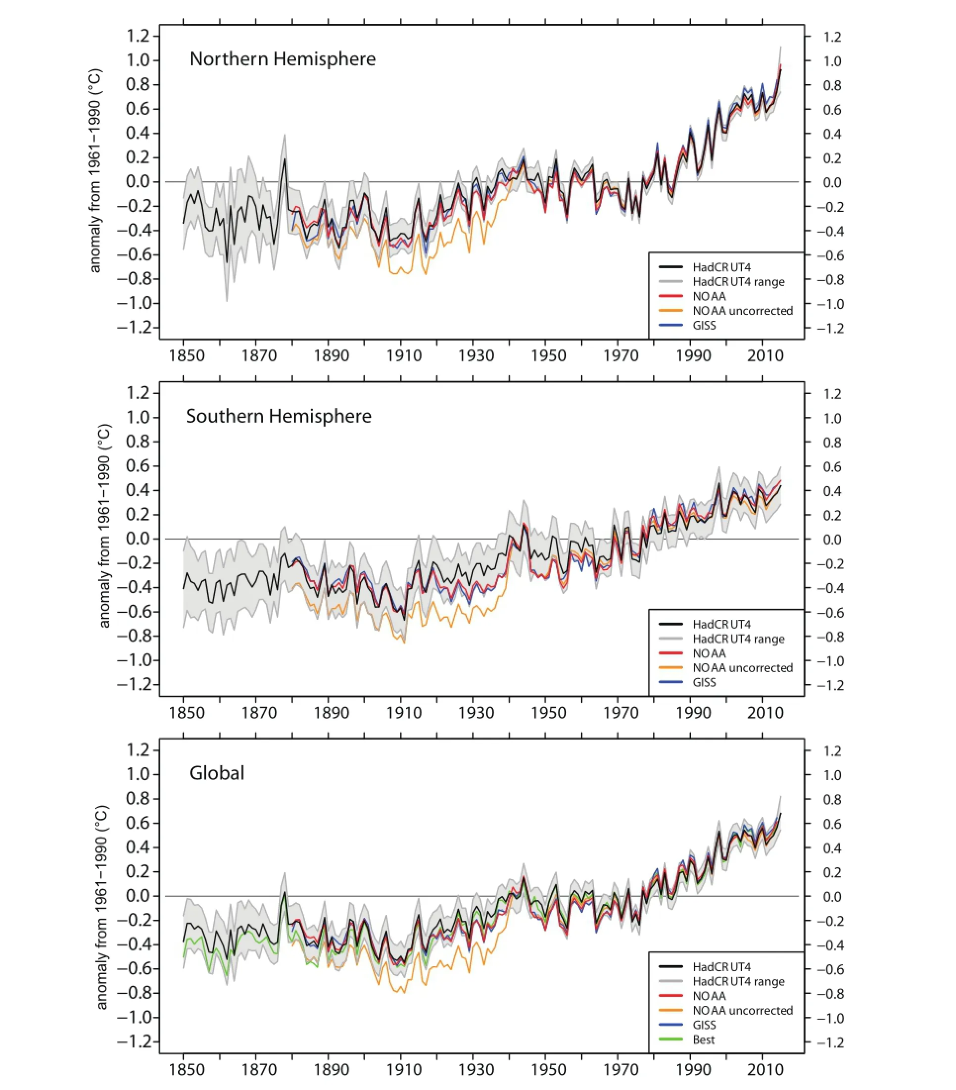
Fig.1. Hemispheric and global averages, based on land and marine data, from the four datasets discussed in this paper: HadCRUT4 (Morice et al., 2012); NCEI/NOAA (Karletal.,2015); GISS (Hansen etal.,2010); and Berkeley Earth (http://berkeleyearth.lbl.gov/auto/Global/LandandOcean summary.txt). The HadCRUT4 range encompasses the 5%and 95%values from their 100 ensembles(Morice et al.,2012).The unadjusted data are from NCEI(Karl et al.,2015).All data are expressed as anomalies from the 1961–90 average.
The global average is(NH+SH)/2,but the greater interannual variability of the NH tends to dominate.BEST is only available for the global average.The BEST series follows HadCRUT4,principally due to their common use of HadSST3 for ocean areas.Despite this,BEST implies cooler temperatures during the period before about 1890—a feature which must be related to cooler land temperature anomalies than HadCRUT4.Finally,the unadjusted NCEI/NOAA data imply much cooler temperatures before 1940,as canvas bucket adjustments were not applied(see also Karl et al., 2015).To further illustrate the importance of the ocean adjustments,Figs.2 and 3 are similar to Fig.1 but show hemispheric and global plots for the land(Fig.2)and marine(Fig. 3)parts of the world.The unadjusted NCEI/NOAA data for the land areas of the world(Fig.2)are not distinguish-able from the CRUTEM4,NCEI/NOAA(adjusted),GISS and BEST time series.Minor differences occur,but they are within the CRUTEM4 5%/95%uncertainty ranges.For marine regions(Fig.3),the unadjusted NCEI/NOAA marine data are clearly offset(for periods before the 1960s)from their adjusted data(ERSSTv4)and HadSST3,and fall outside the 5%/95%uncertainty ranges based on HadSST3.Furthermore,the difference between ERSSTv4 and HadSST3 is quitelargeattimes,particularlyfortheSH(e.g.,forthe1930s and the 1950s)—clear evidence that the uncertainty in SST bias adjustment is much larger than for the terrestrial part of the world in Fig.2.
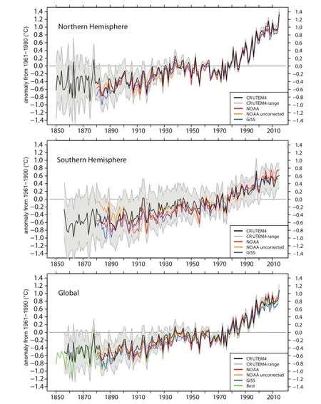
Fig.2.Hemispheric and global averages,based on land data,from the four datasets discussed in this paper:CRUTEM4(Jones et al.,2012);NCEI/NOAA(Karl et al.,2015);GISS(Hansen et al.,2010);and Berkeley Earth(http://berkeleyearth.lbl.gov/regions/global-land).The CRUTEM4 range encompasses the 5%and 95%values from their 100 ensembles(Morice et al.,2012).The unadjusted data are from NCEI(Karl et al.,2015).All data are expressed as anomalies from the 1961–90 average.
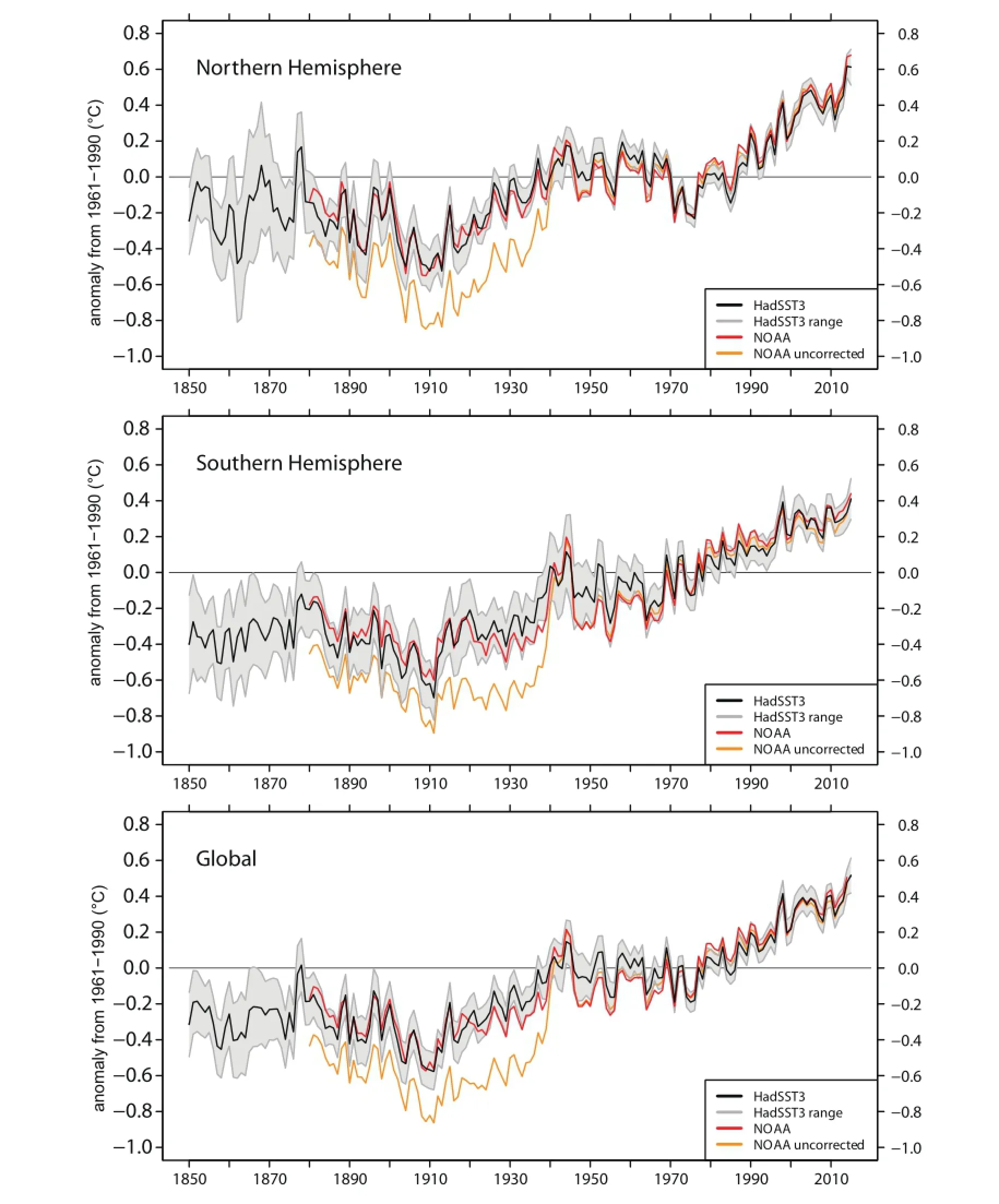
Fig.3.Hemispheric and global averages,based on marine data,from two of the datasets discussed in this paper:HadSST3(Kennedy et al.,2011b)and NCEI/NOAA(Karl et al.,2015).The HadSST3 range encompasses the 5%and 95%values from their 100 ensembles(Morice et al.,2012).The unadjusted data are from NCEI(Karl et al.,2015).All data are expressed as anomalies from the 1961–90 average.
On interannual timescales in all three figures,warm years can be clearly related to El Ni?no years and cool years to La Ni?na years or to large explosive volcanic eruptions in the tropics[see illustrations of this in Foster and Rahmstorf (2011)].The greatest El Ni?no events of the last 200 years occurred in 1877/78 and 1997/98.On longer timescales,the world has warmed in two phases,from about 1920 to the early 1940s and from the late-1970s.The warmest year in all four global records is 2014,but this value only just exceeds that measured in 1998,2005 and 2010.Initial data for 2015, partly due to the current El Ni?no,indicate that 2015 will be significantly warmer than all other years.If the El Ni?no event continues,then it is possible that 2016 will be warmer still.
Finally,in this section,trends are calculated for the globalaverage(from the land and marine datasets)for the four datasets and for NCEI-unadjusted for three different time periods(1901–2014,1951–2014 and 1979–2014).The final period represents the period of satellite coverage.The results are given in Table 1 and all trends are statistically significant at the 99%level for all periods.The NCEI uncorrected series is also included and this clearly shows a greater long-term warming(for 1901–2014)than would have occurred if the bias and homogeneity adjustments were not applied.The results presented here and in Karl et al.(2015)and Kennedy et al.(2011b)clearly show that this is due to the SST bias(see Fig.3).
Much has been written about temperature trends over the past 15 years(often starting during or just after the major El Ni?no event of 1997/98),with the period being referred to as a“hiatus”in warming(e.g.,Hartmann et al.,2013;Karl et al., 2015,and references therein).A number of possible explanations have proposed for this,but Karl et al.(2015)conclude that their new analysis doesn’t support the notion of a hiatus. From a data perspective,this will be further enhanced by the upcoming warm years of 2015 and 2016.As La Ni?na events generally follow El Ni?no events,it is likely that 2017 and 2018 might be cooler.Rather than then starting a new hiatus, it could be beneficial to additionally discuss global average temperatures after the effects of El Ni?no and La Ni?na events have been removed[using approaches similar to Thompson et al.(2009)or Foster and Rahmstorf(2011)].
8.Conclusions
The importance of inhomogeneities in raw surface temperature observations becomes clear when comprehensive models to estimate the uncertainties involved are developed (e.g.,Brohan et al.,2006;Morice et al.,2012;Karl et al., 2015).Factors that affect individual site records tend to be random(i.e.,they can lead to positive or negative biases)and so uncertainties in any adjustments for land stations become less and less important as data are averaged over larger areas. Biases that affect multiple sites or records(such as changing measurement techniques for SSTs,changes in exposure of land stations and urbanization),although smaller in magnitude than many individual land station adjustments,become more important the larger the area averaged.As illustrated by Fig.1,the four groups independently account for all these issues and produce series within the error estimates of Had-CRUT4.Using only unadjusted data,Karl et al.(2015)show that if the biases and homogeneity issues are ignored,the world would have warmed more.This result is primarily due to the SST bucket bias.
The impacts of sparser coverage in early decades are only important before 1880,and,even then,the impact is mostly felt in the Southern Hemisphere(Jones,1994).For the Northern Hemisphere,it is possible to derive reliable hemispheric averages from instrumental data back to about 1850.For example,Karl et al.(1994)show that global 100+year trends become quite reliable after the 1870s based on historical sampling.
Understanding the major sources of inhomogeneity provides key information for reducing uncertainties in hemispheric averages.Uncertainties would be most significantly reduced through the inclusion of more SST data in the 19th centurythanthroughaddingmorelandstationseriessincethe 1950s.A number of current projects are seeking to digitize much of the British logbook material available in archives. The potential size and importance of SST data,also requires enhancements to our knowledge of how SST and MAT measurements were taken in the past(Kent et al.,2010;Kennedy, 2014).More SST data are not only important for improving the reliability of hemispheric and global temperature series,but can help to improve infilled SST fields,which are vital for extended reanalyses.For terrestrial regions,adding more land stations can also help reduce uncertainties,but emphasis needs to be focussed on regions with sparse coverage,as opposed to simply increasing station numbers in wellmonitored regions.For identifying past large-scale changes in temperature at the Earth’s surface,however,the homogenized datasets currently available provide highly reliable information back into the 19th century and show unequivocally that the world has warmed considerably over this period.
Open Access This article is distributed under the terms of the Creative Commons Attribution 4.0 International License(http://creativecommons.org/licenses/by/4.0/),which permits unrestricted use,distribution,and reproductioninany medium,provided you give appropriate credit to the original author(s)and the source,provide a link to the Creative Commons license,and indicate if changes were made.
REFERENCES
Arnfield,A.J.,2003:Two decades of urban climate research:a review of turbulence,exchanges of energy and water,and the urban heat island.Inter.J.Climatol.,23,1–26.
B¨ohm,R.,P.D.Jones,J.Hiebl,D.Frank,M.Brunetti,and M. Maugeri,2010:The early instrumental warm-bias:A solution for long Central Europe an temperature series 1760–2007.Climatic Change,101,41–67.
Bojinski,S.,M.Verstraete,T.C.Peterson,C.Richter,A.Simmons,and M.Zemp,2014:The concept of essential climate variablesinsupport ofclimateresearch,applications,andpolicy.Bull.Amer.Meteor.Soc.,95,1431–1443.
Brohan,P.,J.J.Kennedy,I.Harris,S.F.B.Tett,and P.D.Jones, 2006:Uncertainty estimates in regional and global observed temperature changes:A new data set from 1850.J.Geophys. Res.,111,D12106,doi:10.1029/2005JD006548.
Brunet,M.,and Coauthors,2011:The minimization of the screen bias from ancient Western Mediterranean air temperature records:an exploratory statistical analysis.Inter.J.Climatol., 31,1879–1895,doi:10.1002/joc.2192.
Callendar,G.S.,1938:The artificial production of carbon dioxide and its influence on temperature.Quart.J.Roy.Meteor.Soc., 64,223–240,doi:10.1002/qj.49706427503.
Callendar,G.S.,1961:Temperature fluctuations and trends over the earth.Quart.J.Roy.Meteor.Soc.,87,1–12,doi:10.1002/ qj.49708737102.
Compo,G.P.,and Coauthors,2011:The twentieth century reanalysis project.Quart.J.Roy.Meteor.Soc.,137,1–28,doi: 10.1002/qj.776.
Compo,G.P.,P.D.Sardesmukh,J.S.Whitaker,P.Brohan,P. D.Jones,and C.McColl,2013:Independent confirmation of global land warming without the use of station.Geophys.Res. Lett.,40,3170–3174,doi:10.1002/grl.50425.
Conrad,V.,and L.W.Pollak,1962:Methods in Climatology.Harvard University Press,459 pp.
Cowtan,K.,and R.G.Way,2014:Coverage bias in the hadcrut4 temperature series and its impact on recent temperature trends.Quart.J.Roy.Meteor.Soc.,140,1935–1944,doi: 10.1002/qj.2297.
Dee,D.P.,and Coauthors,2011:The ERA-Interim reanalysis: configuration and performance of the data assimilation system.Quart.J.Roy.Meteor.Soc.,137,553–597,doi:10.1002/ qj.828.
Farmer,G.,T.M.L.Wigley,P.D.Jones,and M.Salmon,1989: Documenting and explaining recent global-mean temperature changes.Final Report to the Natural Environment Research Council,Contract No.GR3/6565,East Anglia University, Norwich,UK.[Available online at http://www.cru.uea.ac. uk/cru/pubs/pdf/Farmer-1989-NERC.pdf.]
Folland,C.K.,2005:Assessing bias corrections in historical sea surface temperature using a climate model.Inter.J.Climatol., 25,895–911,doi:10.1002/joc.1171.
Folland,C.K.,and D.E.Parker,1995:Correction of instrumental biases in historical sea surface temperature data.Quart.J. Roy.Meteor.Soc.,121,319–367.
Foster,G.,and S.Rahmstorf,2011:Global temperature evolution 1979-2010.Environ.Res.Lett.,6,044022,doi: 10.1088/1748-9326/6/4/044022.
Hansen,J.,R.Ruedy,J.Glascoe,and M.Sato,1999:GISS analysis of surface temperature change.J.Geophys.Res.,104, 30 997–31 022,doi:10.1029/1999JD900835.
Hansen,J.,M.Sato,R.Ruedy,K.Lo,D.W.Lea,and M.Medina-Elizade,2006:Global temperature change.Proceedings of the National Academy of Sciences of the United States of America,103,14 288–14 293.
Hansen,J.,R.Ruedy,M.Sato,and K.Lo,2010:Global surface temperature change.Rev.Geophys.,48,RG4004,doi: 10.1029/2010RG000345.
Hartmann,D.L.,and Coauthors,2013:Observations:Atmosphere and surface.Climate Change 2013:The Physical Science Basis.Contribution of Working Group I to the Fifth Assessment Report of the Intergovernmental Panel on Climate Change,T. F.Stocker et al.,Eds.Cambridge University Press.
Hawkins,E.,and P.D.Jones,2013:On increasing global temperatures:75 years after Callendar.Quart.J.Roy.Meteor.Soc., 139,1961–1963,doi:10.1002/qj.2178.
Hersbach,H.,C.Peubey,A.Simmons,P.Berrisford,P.Poli,and D.Dee,2015:ERA-20CM:A twentieth-century atmospheric model ensemble.Quart.J.Roy.Meteor.Soc.,141,2350–2375,doi:10.1002/qj.2528.
Huang,B.Y.,and Coauthors,2015:Extended reconstructed Sea surface temperature Version 4(ERSST.v4).Part I:upgrades and intercomparisons.J.Climate,28,911–930.
Ishii,M.,A.Shouji,S.Sugimoto,and T.Matsumoto,2005:Objective analyses of Sea-surface temperature and marine meteorological variables for the 20th century using ICOADS and the Kobe collection.Inter.J.Climatol.,25,865–879.
Jansen,E.,and Coauthors,2007:Palaeoclimate.Climate Change 2007:The Physical Science Basis.Contribution of Working Group I to the Fourth Assessment Report of the Intergovernmental Panel on Climate Change,S.Solomon et al.,Eds. Cambridge University Press,433–497.
Jones,P.D.,1994:Hemispheric surface air temperature variations: a reanalysis and an update to 1993.J.Climate,7,1794–1802.
Jones,P.D.,and D.H.Lister,2009:The urban heat island in central London and urban-related warming trends in central London since 1900.Weather,64,323–327.
Jones,P.D.,and D.H.Lister,2015:Antarctic near-surface air temperatures compared with ERA-Interim values since 1979. International Journal of Climatology,35,1354–1366,doi: 10.1002/joc.4061.
Jones,P.D.,and T.M.L.Wigley,2010:Estimation of global temperature trends:What’s important and what isn’t.Climatic Change,100,59–69.
Jones,P.D.,P.Y.Groisman,M.Coughlan,N.Plummer,W.-C. Wang,and T.R.Karl,1990:Assessment of urbanization effects in time series of surface air temperature over land.Nature,347,169–172.
Jones,P.D.,T.J.Osborn,and K.R.Briffa,1997:Estimating sampling errors in large-scale temperature averages.J.Climate, 10,2548–2568.
Jones,P.D.,K.R.Briffa,and T.J.Osborn,2003:Changes in the Northern hemisphere annual cycle:Implications for paleoclimatology?J.Geophys.Res.,108,4588,doi:10.1029/2003JD 003695.
Jones,P.D.,D.H.Lister,and Q.Li,2008:Urbanization effects in large-scale temperature records,with an emphasis on China. J.Geophys.Res.,113,D16122,doi:10.1029/2008JD009916.
Jones,P.D.,D.H.Lister,T.J.Osborn,C.Harpham,M.Salmon, and C.P.Morice,2012:Hemispheric and large-scale landsurface air temperature variations:An extensive revision and an update to 2010.J.Geophys.Res.,117,D05127,doi: 10.1029/2011JD017139.
Kalnay,E.,and Coauthors,1996:The NCEP/NCAR 40-year reanalysis project.Bull.Amer.Meteor.Soc.,77,437–471.
Karl,T.R.,C.N.Williams Jr.,P.J.Young,and W.M.Wendland, 1986:A model to estimate the time of observation bias associated with monthly mean maximum,minimum and mean temperatures for the United States.J.Climate Appl.Meteor., 25,145–160.
Karl,T.R.,R.W.Knight,and J.R.Christy,1994:Global and hemispheric temperature trends:Uncertainties related to inadequate spatial sampling.J.Climate,7,1144–1163.
Karl,T.R.,and Coauthors,2015:Possible artifacts of data biasesintherecentglobalsurfacewarminghiatus.Science,348, 1469–1472.
Kennedy,J.J.,2014:A review of uncertainty in in situ measurements and data sets of Sea surface temperature.Rev.Geophys.,52,1–32,doi:10.1002/2013RG000434.
Kennedy,J.J.,N.A.Rayner,R.O.Smith,D.E.Parker,and M. Saunby,2011a:Reassessing biases and other uncertainties in Sea surface temperature observations measured in situ since 1850:1.Measurement and sampling uncertainties.J.Geophys.Res.,116,doi:10.1029/2010JD015218.
Kennedy,J.J.,N.A.Rayner,R.O.Smith,D.E.Parker,and M. Saunby,2011b:Reassessing biases and other uncertainties in Sea surface temperature observations measured in situ since 1850:2.Biases and homogenization.J.Geophys.Res.,116, doi:10.1029/2010JD015220.
Kent,E.C.,J.J.Kennedy,D.I.Berry,and R.O.Smith,2010:Ef-fects of instrumentation changes on sea surface temperature measured in situ.Wiley Interdisciplinary Reviews:Climate Change,1(5),718–728,doi:10.1002/wcc.55.
Kent,E.C.,N.A.Rayner,D.I.Berry,M.Saunby,B.I.Moat,J. J.Kennedy,and D.E.Parker,2013:Global analysis of night marine air temperature and its uncertainty since 1880:The HadNMAT2 data set.J.Geophys.Res.,118,1281–1298,doi: 10.1002/jgrd.50152.
K¨oppen,W.,1873:¨Uber mehrj¨ahrige perioden der witterung, insbesondere¨uber die 11-j¨ahrige periode der temperatur. Zeitschrift der¨Osterreichischen Gesellschaft f¨ur Meteorologie,Bd VIII,241–248,257–267.
Le Treut,H.,R.Somerville,U.Cubasch,Y.Ding,C.Mauritzen, A.Mokssit,T.Peterson,and M.Prather,2007:Historical overview of climate change.Climate Change 2007:The Physical Science Basis.Contribution of Working Group I to the Fourth Assessment Report of the Intergovernmental Panel on Climate Change,S.Solomon et al.,Eds.Cambridge University Press,Cambridge,United Kingdom and New York, NY,USA,93–127.
Li,Q.X,J.Y.Huang,Z.H.Jiang,L.M.Zhou,P.Chu,and K. X.Hu,2014:Detection of urbanization signals in extreme winter minimum temperature changes over Northern China. Climatic Change,122,595–608.
Liu,W.,and Coauthors,2015:Extended reconstructed Sea surface temperature Version 4(ERSST.v4):Part II.Parametric and structural uncertainty estimations.J.Climate,28,931–951.
Lugina,K.M.,P.Y.Groisman,K.Y.Vinnikov,V.V.Koknaeva, and N.A.Speranskaya,2006:Monthly surface air temperature time series area-averaged over the 30-degree latitudinal belts of the globe,1881–2005.Trends:A Compendium of Data on Global Change.Carbon Dioxide Information Analysis Center,Oak Ridge National Laboratory,U.S.Dept.Energy,Oak Ridge,Tenn.,U.S.A.[Available online at http:// cdiac.esd.ornl.gov/trends/temp/lugina/lugina.html.]
Masson-Delmotte,V.M.,and Coauthors,2013:Information from paleoclimate archives.Climate Change 2013:The Physical Science Basis.Contribution of Working Group I to the Fifth AssessmentReportoftheIntergovernmentalPanelonClimate Change,T.F.Stocker et al.,Eds.Cambridge University Press, Cambridge,United Kingdom and New York,NY,USA.
Maury,M.F.,1855:Wind and Current Charts.7th ed.,US Navy, Philadelphia.
Menne,M.J.,C.N.Williams Jr.,and R.S.Vose,2009:The U.Shistoricalclimatologynetworkmonthlytemperaturedata, Version 2.Bull.Amer.Meteor.Soc.,90,993–1007.
Moberg,A.,H.Alexandersson,H.Bergstr¨om,and P.D.Jones, 2003:Were southern Swedish summer temperatures before 1860 as warm as measured?Inter.J.Climatol.,23,1495–1521.
Morice,C.P.,J.J.Kennedy,N.A.Rayner,and P.D.Jones,2012: Quantifying uncertainties in global and regional temperature change using an ensemble of observational estimates:the HadCRUT4 data set.J.Geophys.Res.,117,D08101,doi: 10.1029/2011JD017187.
Nicholls,N.,R.Tapp,K.Burrows,and D.Richards,1996:Historical thermometer exposures in Australia.Inter.J.Climatol., 16,705–710.
Parker,D.E.,1994:Effects of changing exposure of thermometers at land stations.Inter.J.Climatol.,14,1–31.
Parker,D.E.,2004:Climate:large-scale warming is not urban. Nature,432,290 pp.
Parker,D.E.,2006:A demonstration that large-scale warming is not urban.J.Climate,19,2882–2895.
Parker,D.E.,2010:Urban heat island effects on estimates of observed climate change.Wiley Interdisciplinary Reviews:Climate Change,1(1),123–133,doi:10.1002/wcc.21.
Parker,D.E.,2011:Recent land surface air temperature trends assessed using the 20th century reanalysis.J.Geophys.Res., 116,D20125,doi:10.1029/2011JD016438.
Parker,D.E.,P.Jones,T.C.Peterson,and J.Kennedy,2009: Comment on“Unresolved issues with the assessment of multidecadal global land surface temperature trends”by Roger A. Pielke Sr.et al.J.Geophys.Res.,114,D05104,doi:10.1029/ 2008JD010450.
Peterson,T.C.,and T.W.Owen,2005:Urban heat island assessment:metadata are important.J.Climate,18,2637–2646.
Poli,P.,and Coauthors,2013:The data assimilation system and initial performance evaluation of the ECMWF pilot reanalysis of the 20th-century assimilating surface observations only (ERA-20C).ERA Report Series,14 pp.
Quayle,R.G.,D.R.Easterling,T.R.Karl,and P.Y.Hughes,1991: Effects of recent thermometer changes in the cooperative station network.Bull.Amer.Meteor.Soc.,72,1718–1723.
Ren,G.Y.,Y.Q.Zhou,Z.Y.Chu,J.X.Zhou,A.Y.Zhang,J. Guo,and X.F.Liu,2008:Urbanization effects on observed surface air temperature trends in North China.J.Climate,21, 1333–1348.
Rennie,J.,and Coauthors,2014:The international surface temperatureinitiativegloballandsurfacedatabank:Monthlytemperature data release description and methods.Geoscience Data Journal,1,75–102,doi:10.1002/gdj3.8.
Rohde,R.,and Coauthors,2013a:A new estimate of the average earth surface land temperature spanning 1753 to 2011. Geoinfor Geostat:An Overview,1,doi:10.4172/2327-4581. 1000101.
Rohde,R.,and Coauthors,2013b:Berkeley earth temperature averaging process.Geoinfor Geostat:An Overview,1,doi: 10.4172/gigs.1000103.
Simmons,A.J.,K.M.Willett,P.D.Jones,P.W.Thorne,and D.P.Dee,2010:Low-frequency variations in surface atmospheric humidity,temperature,and precipitation:inferences from reanalyses and monthly gridded observational data sets. J.Geophys.Res.,115,D01110,doi:10.1029/2009JD012442. Smith,T.M.,R.W.,and Reynolds,2005:A global merged land andseasurfacetemperaturereconstructionbasedonhistorical observations(1880–1997).J Climate,18,2021–2036.
Smith,T.M.,R.W.Reynolds,T.C.Peterson,and J.Lawrimore, 2008:Improvements to NOAA’s historical merged Land-Ocean surface temperature analysis(1880–2006).J.Climate, 21,2283–2293.
Thompson,D.W.J.,J.J.Kennedy,J.M.Wallace,and P.D.Jones, 2008:A large discontinuity in the mid-twentieth century in observed global-mean surface temperature.Nature,453,646–649.
Thompson,D.W.J.,J.M.Wallace,P.D.Jones,and J.J.Kennedy, 2009:Identifying signatures of natural climate variability in timeseriesofglobal-meansurfacetemperature:Methodology and insights.J.Climate,22,6120–6141.
Trenberth,K.E.,and Coauthors,2007:Observations:surface and atmospheric climate change.Climate Change 2007:The Physical Science Basis.Contribution of Working Group 1 to the Fourth Assessment Report of the Intergovernmental Panel on Climate Change,S.D.Solomon et al.,Eds.CambridgeUniversity Press,235–336.
Trewin,B.,2010:Exposure,instrumentation,and observing practice effects on land temperature measurements.Wiley Interdisciplinary Reviews:Climate Change,1,490–506,doi: 10.1002/wcc.46,2010.
Venema,V.K.C.,and Coauthors,2012:Benchmarking homogenization algorithms for monthly data.Climates of the Past,8, 89–115.
Vose,R.S.,and Coauthors,2012:NOAA’s merged Land–Ocean surface temperature analysis.Bull.Amer.Meteor.Soc.,93, 1677–1685,doi:10.1175/BAMS-D-11-00241.1.
Wang,F.,Q.S.Ge,S.W.Wang,Q.X.Li,and P.D.Jones, 2015:A new estimation of urbanization’s contribution to the warming trend in China.J.Climate,28,8923–8938,doi: 10.1175/JCLI-D-14-00427.1.
Wang,J.,Z.W.Yan,P.D.Jones,and J.J.Xia,2013:On“observation minus reanalysis”method:A view from multidecadal variability.J.Geophys.Res.,118,7450–7458,doi:10.1002/ jgrd.50574.
Wickham,C.,and Coauthors,2013:Influence of urban heating on the global temperature land average using rural sites identified from MODIS classifications.Geoinfor Geostat:An Overview,1,doi:10.4172/2327-4581.1000104.
Wilby,R.L.,P.D.Jones,and D.H.Lister,2011:Decadal variations in the nocturnal heat island of London.Weather,66, 59–64.
Woodruff,S.D.,and Coauthors,2011:ICOADS release 2.5: extensions and enhancements to the surface marine meteorological archive.Inter.J.Climatol.,31,951–967,doi: 10.1002/joc.2103.
Xu,W.H.,Q.X.Li,X.L.Wang,S.Yang,L.J.Cao,and Y.Feng, 2013:Homogenization of Chinese daily surface air temperatures and analysis of trends in the extreme temperature indices.J.Geophys.Res.,118,9708–9720,doi:10.1002/jgrd. 50791.
Zhao,P.,P.D.Jones,L.J.Cao,Z.W.Yan,S.Y.Zha,Y.N.Zhu, Y.Yu,and G.L.Tang,2014:Trend of surface air temperature in eastern china and associated large-scale climate variability over the last 100 years.J.Climate.27,4693–4703,doi: 10.1175/JCLI-D-13-00397.1.
Zhou,L.M.,R.E.Dickinson,Y.H.Tian,J.Y.Fang,Q.X.Li,R.K. Kaufmann,C.J.Tucker,and R.B.Myneni,2004:Evidence for a significant urbanization effect on climate in China.Proceedings of the National Academy of Sciences of the United States of America,101,9540–9544.
Jones,P.,2016:The reliability of global and hemispheric surface temperature records.Adv.Atmos.Sci.,33(3), 269–282,
10.1007/s00376-015-5194-4.
?Philip JONES
Email:P.Jones@uea.ac.uk
 Advances in Atmospheric Sciences2016年3期
- Advances in Atmospheric Sciences的其它文章
- Land Response to Atmosphere at Different Resolutions in the Common Land Model over East Asia
- A Global Spectral Element Model for Poisson Equations and Advective Flow over a Sphere
- Climatology of Lightning Activity in South China and Its Relationships to Precipitation and Convective Available Potential Energy
- Weak ENSO Asymmetry Due to Weak Nonlinear Air-Sea Interaction in CMIP5 Climate Models
- Assessment of Interannual Sea Surface Salinity Variability and Its Effects on the Barrier Layer in the Equatorial Pacific Using BNU-ESM
- Phase Transition of the Pacific Decadal Oscillation and Decadal Variation of the East Asian Summer Monsoon in the 20th Century