Improved conservative level set method for free surface flow simulation*

ZHAO Lan-hao (趙蘭浩), MAO Jia (毛佳), LIU Xiao-qing (劉曉青)

College of Water Conservancy and Hydropower Engineering, Hohai University, Nanjing 210098, China, E-mail: zhaolanhao@hhu.edu.cn

BAI Xin, WILLIAMS J. J. R.

School of Engineering and Materials Science, Queen Mary University of London, London, UK

Improved conservative level set method for free surface flow simulation*

ZHAO Lan-hao (趙蘭浩), MAO Jia (毛佳), LIU Xiao-qing (劉曉青)

College of Water Conservancy and Hydropower Engineering, Hohai University, Nanjing 210098, China, E-mail: zhaolanhao@hhu.edu.cn

BAI Xin, WILLIAMS J. J. R.

School of Engineering and Materials Science, Queen Mary University of London, London, UK

(Received December 17, 2013, Revised January 16, 2014)

By coupling the standard and the conservative level set methods, an improved conservative level set method is proposed to capture the free surface smoothly with excellent mass conservation properties. The improvement lies in the fact that the surface normal is computed from a signed distance function instead of the Heaviside function. Comparing with the conservative level set method, the inevitable numerical discretization errors to point the surface normal in arbitrary directions could be eliminated, and the instability of the numerical solution could be improved efficiently. The advantage is clear in the straightforward combination of the standard level set and the conservative level set and a little effort is taken in coding compared with other coupled methods. The present method is validated with several well-known benchmark problems, including the 2-D Zalesak’s disk rotating, the 3-D sphere stretching in deformation vortex and the dam break flow simulation. The results are shown to be in good agreement with the published experimental data and numerical results.

free surface flow, improved conservative level set, mass conservation

Introduction

The numerical simulation of a free surface flow is of great importance in the field of computational fluid dynamics (CFD) with a great number of applications in civil, coastal, offshore engineerings. The difficulties of this problem are due to the existence of the arbitrarily moving boundary, especially, involving the interface break-up, mixing or the entrapment of one fluid within another.

Depending upon how the interface is described, the numerical methods for the free surface flow simulation in the Eulerian frame generally fall into two categories, the interface tracking and the interface capturing[1]. In the interface tracking, the interface is represented and tracked explicitly either by special marker points or attached to a surface mesh[2]. The difficulty in handling drastic changes in the interface topology is due to an inherent weakness of the interface tracking method.

In contrast, the interface capturing methods have gained more popularity for their capability of naturally dealing with complex topological changes. Rather than tracking the interface explicitly, those methods rely on an implicit representation of the interface with an indicator function. Among them, the volume of fluid (VOF) method[3]and the level set (LS) method are most popular. The LS method enjoys considerable popularity since it was introduced by Osher and Sethian due to its simplicity and ability to capture the interfaces. One of the advantages is that it can handle the merging and breaking of the interfaces automatically, so the interface never has to be explicitly reconstructed as in the case of the VOF method. Owing to the smooth nature of the signed distance functions, both the unit normal and the curvature of the interface can be easily transported and accurately calculated.However, it has a severe drawback related with the mass conservation. As time evolves, even a negligibly small error can be accumulated to a sufficiently large magnitude and may finally lead to the breaking down of the solution[4].

Many attempts were made to improve the mass conservation of the LS methods, but the mass conservation is never exactly reached[5]. The other approaches to deal with this problem are to couple the LS method with other methods such as the particle level set (PLS) method[6,7]and the coupled level set/VOF (CLSVOF) method[8]. Although all coupled methods might significantly improve the original method in certain aspects, the coupling introduces additional problems. Their cost is typically greater than the cost of a simple LS method, and the original simplicity of the LS methods is partly lost.

On the other hand, the conservative level set (CLS) method proposed by Elin et al.[9,10]improves the mass conservation and retains the simplicity of the original method at the same time. Compared with the standard LS method, the CLS method drastically improves the mass conservation properties and has been successfully employed in many applications[11-13]. With the CLS method, the shape and the width of the profile across the interface should be kept constant all time and hence a re-initialization process is essential. During the re-initialization, the compression part and the diffusion part are iteratively updated until a steady state is reached. As both the compression and the diffusion take place only in the normal direction of the interface, an inaccurate approximation of the interface normal vectors will affect the mass conservation property and even cause the problem to collapse. The normal or the curvature of the interface cannot be calculated as accurate as with the LS method. Far away from the interface, the gradient of the smeared Heaviside function for the CLS method will be very small and hence the direction of the normal will be extremely sensitive to small spurious errors. Such errors are inevitable in a general numerical discretization and will cause the normal vectors pointing in arbitrary directions and eventually lead to the instability of the numerical solution. This problem was emphasized in literature[14].

In this paper, the conservative level set method for the free surface flow simulation is improved with respect to the problems mentioned above. The basic idea is related to the fact that the standard LS method can provide a smooth geometrical information of the interface but without a satisfactory mass conservation, while the CLS method ensures a good mass conservation if an accurate interface normal direction is given. In the present approach, the CLS method is employed to capture the interfaces, with good mass conservation properties, and the standard LS method is used to give the accurate surface information. The technique is called the improved conservative level set (ICLS) method. Moreover, unlike other coupling techniques, the methodology behind the CLS and the LS methods is essentially identical, and the ICLS can be implemented in a straightforward manner while still retaining the simplicity of the original method.

The paper proposes an improvement of the conservative level set method and use it for the free surface flow simulation. The improvement of the method lies in the fact that the surface normal is computed from a signed distance function instead of using the Heaviside function. The present ICLS method can capture the free surface smoothly with excellent mass conservation properties. Based on the basic idea of the standard LS and the CLS methods, the methodology of the ICLS method is discussed. And then the ICLS method is coupled with the Navier-Stokes equation to simulate the free surface flow. Finally, several challenging benchmark test cases are simulated to validate the proposed technique, and excellent mass conservation properties and smoother interface are shown.

1. Motivation and methodology

1.1 Basic idea of the standard level set method

In the standard LS method, the level set function φ is defined as the signed distance to the interface Γ

The value of φ is set as positive in one side and negative in the other, with the zero level set of φ indicating the interface

For two incompressible fluids separated by the interface Γ in a domain Ω, the level set function is advected by the fluid velocity field u

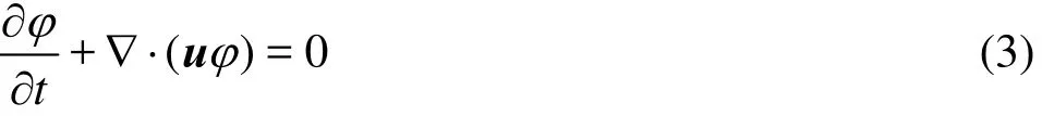
To capture the interface accurately, the level set function must be a distance function, that is,=1. However, due to the fact that the velocity field is not a simple uniform one and may vary rapidly because φ will generally drift away from its initialized value as a signed distance during the evolving interface. To keep φ as a distance function, a re-initialization equation proposed by Sussman is traditionally iterated for a few steps in fictitious time τ

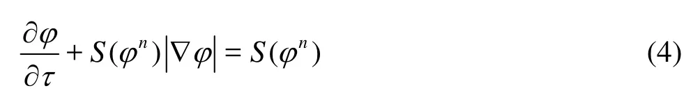
where S() is the sign function.

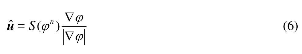
Equation (4) can also be written as

And it is shown that this problem consists of advecting φ by a velocity field

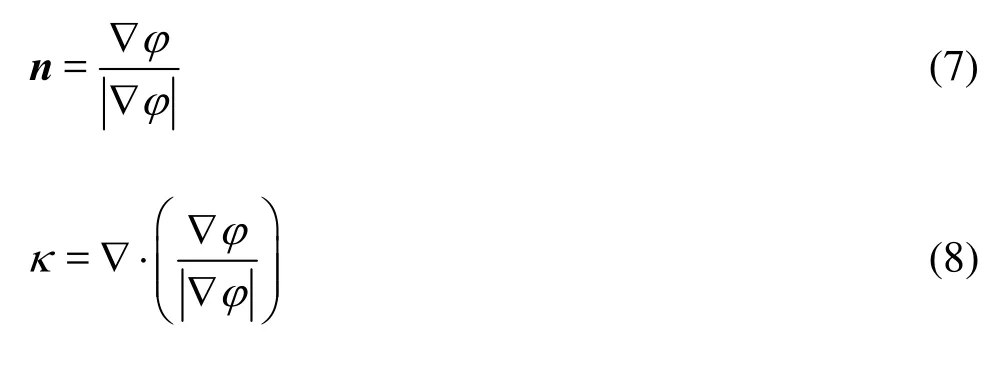
The geometric properties, including the normal vector and the curvature, can be estimated readily from the level set function:

1.2 Conservative level set method

The most notable difference between the CLS method originally proposed by Elin et al.[9,10]and the standard LS method lies in the choice of the level set function. Instead of the signed distance function, the CLS method employs the Heaviside function:

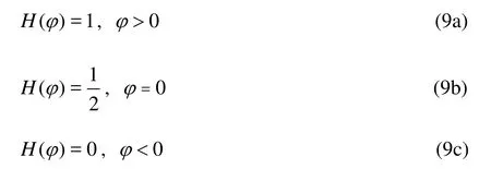
where φ is the signed distance function as in the LS method.

The strong discontinuity of material properties at the interface due to the great difference between the air and the water will cause instability of the numerical solutions. In practice, a hyperbolic tangent function H is often employed as the level set function for the CLS method

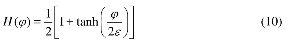
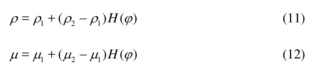
where ε defines a spreading width of H. The material properties such as the density ρ and the viscosity μ are then computed as follows:

The total mass for one of the fluids is given as follows

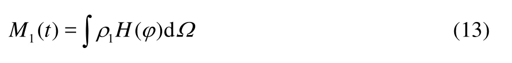
And the conservation of the fluid mass implies the following equation

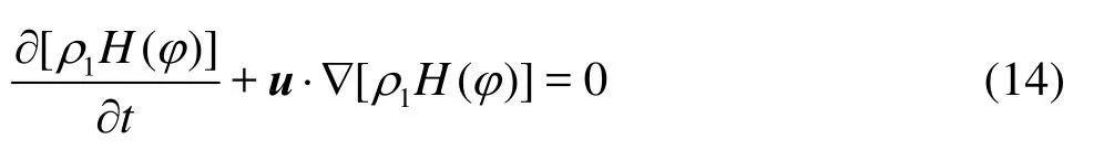
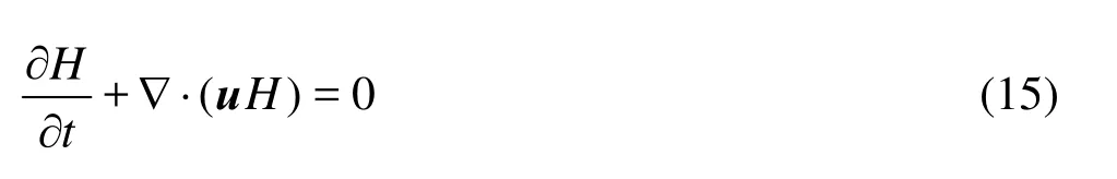
By introducing the continuity equation for incompressible flow, the level set equation can be written in a conservative way

Due to the existence of inevitable numerical errors or artificial diffusions together with velocity variations, the shape of H across the interface will be distorted when H is advected. Thus, a re-initialization step is necessary to maintain the shape and the width of the interface

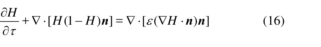
where n is the normal vector at the beginning of the re-initialization, and ε determines the width of the interface. It is important to mention that the re-initialization equation should also be in a conservative form. In Eq.(16), the flux term on the left-hand-side causes a compression of the interface profile, while the righthand-side term is a diffusive flux. When Eq.(16) is evolved to a steady state with fictitious time τ, the diffusion in the normal direction of the interface is balanced by the compressive term, and the shape and the width of the interface are well maintained, which is compulsory for the conservative property.

Although the geometric properties, such as n, can also be estimated from the conservative level set function, a special attention should be paid to such approximation due to the difference between H and φ. This problem is discussed in detail in the next section.

1.3 Improved conservative level set method

1.3.1 Interface normal vector

It can be easily seen from Eq.(16) that the normal vector of the interface plays an important role in the re-initialization since both the compression and the diffusion take place only in the normal direction. An inaccurate interface normal vector will affect the mass conservation property and even destroy the solution.

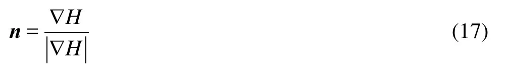
As mentioned by Olsson and Kreiss[9]and Olsson et al.[10], the normal vector for the CLS method can be computed in a convenient way as

However, this approach is strongly sensitive to spurious oscillations in the H field[14]. In fact, although the conservative level set function H is as smooth as the standard level set function φ, the normal or the curvature of the interface cannot be calculated with the same order of accuracy. According to Eq.(10) and considering φ as a signed distance function, i.e.,=1, the gradient modulus of H can be written as

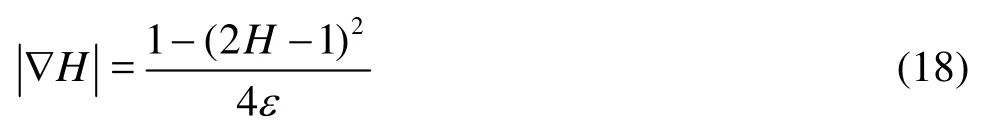
From Eq.(18), it is clear that away from the interface, the gradient of the smeared Heaviside function will be very small because the value of H is close to 0 or 1. As a result, the direction of the normal will be extremely sensitive to small spurious errors which are inevitable in a general numerical discretization, and hence the resulting normal would point in an arbitrary direction. Such arbitrary normal pointing towards each other will lead to severe numerical difficulties. The normal vector obtained by Eq.(17) is not appropriate to be used in the re-initialization equation. For instance, the unphysical accumulation of H would be created during the re-initialization where the normal vectors are facing each other.

One possible way to remedy this issue is to reconstruct a signed distance function φ from the inverse of Eq.(10) using the Heaviside function H, and the normal vectors are computed from Eq.(7) after φ is re-initialized. The overall robustness is increased by this strategy. However, the reconstructed signed distance function itself is also extremely sensitive to small spurious errors, especially at the boundary of the interface. This can be easily verified from the inverse of Eq.(10), φ=εln[H/(1-H )] in which a trivial variation in H can cause an enormous error in φ when the value of H is near 0 or 1.

1.3.2 Improvement strategy

Based on the above discussions, the proposed ICLS method is a hybrid numerical scheme combining the LS and CLS methods. In the ICLS method, the CLS method is used to advect and capture the interfaces, while the standard LS method is employed to give the accurate surface normal approximations.

The merit of the present method lies in the approach to approximate the interface normal vectors. Unlike the conservative LS method, the normal vectors are computed from the signed distance function φ instead of the Heaviside function H. Moreover, to avoid the enormous errors introduced by calculating φ from the reverse of H the signed distance function is advected by Eq.(3) and re-initialized by Eq.(4) in the same manner as the traditional LS method. However, during the re-initialization of the signed distance function, a considerable motion of the zero level set can occur, which can lead to a wrong interface location. To avoid this problem, the signed distance for points closest to the interface are not updated until the end of the time step, this means that the points whosevalues below a certain threshold level δ are excluded from the re-initialization. Similarly, the normal vectors for such points are obtained from the Heaviside function H while the rest are from the re-initialized signed distance function φ Having obtained all normal vectors, the Heaviside function is implicitly re-initialized until a steady state of the interface is reached. At the end of each time step, the signed distance of these excluded points can simply be updated by the inverse of Eq.(10) and carried into the next time step. Since the value of H for the points close to the interface is about 0.5, this procedure will not amplify the spurious errors.

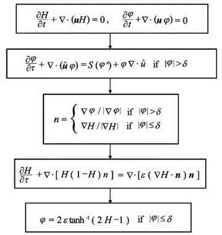
Fig.1 Flow chart of the proposed ICLS method

Following the improvement strategy discussedabove, the flow chart of the proposed ICLS method is shown in Fig.1.

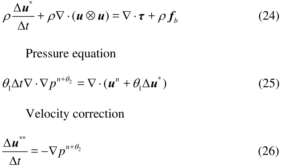
2. Coupling with navier-stokes equations

The determination of the unsteady, viscid and incompressible flow of two interacting fluids requires the solution of the Navier-Stokes equations:

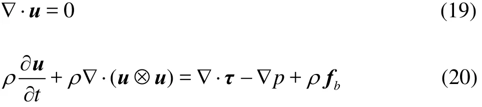
where t is the time, ? is the gradient operator, u is the velocity, τ=μ(?u+?Tu) is the viscous term, p is the pressure and fbis the body force (only the gravity is taken into account here). The density ρ and the dynamic viscosity μ are determined by Eqs.(11) and (12), respectively.

Two parameters, 1θ and 2θ are introduced to represent the time stepping and the governing equations are rewritten in the following time discretized form:

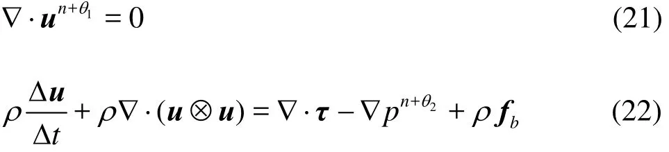
where the parameters1θ and2θ can be chosen in the range [0,1]. Both1θ and2θ are set to 1.0 in the numerical experiments in the next section.

Following the fractional step procedure, the increment Δu can be decomposed into two parts

The discretization of the incompressible Navier-Stokes equations can be split into three stages, i.e.,

Intermediate velocity increment

The two-step Taylor-Galerkin (TSTG) scheme is employed in this paper to discretize both the Navier-Stokes equations and the level set equations. The TSTG is developed from the traditional TG method. It has the advantage of being easy to program together with high efficiency and has been successfully employed in many applications.

The proposed algorithm for solving the free surface flows with the ICLS method is summarized below. For each time step the following steps are executed:

(1) Calculate φn,*, Hn,*using Eqs.(3) and (15), respectively.

(2) Solve Eq.(5) to reach a steady state with φn,*as the initial data. This gives φn+1and in case of＞δ, φn+1=φn ,*.

(3) Calculate n from φn+1using Eq.(7) in case of＞δ, otherwise calculate n from Hn,*using Eqs.(7) and (17).

(4) Solve Eq.(16) to reach a steady state with Hn,*as the initial data, this gives Hn+1.

(5) Update φn+1from Hn+1by the inverse of Eq.(10) in case of≤δ.

(6) Calculate material properties fromn+1H.

(7) Calculate intermediate velocityn,*u from Eq.(24).

(8) Calculaten+1p from Eq.(25).

(9) Perform the velocity correction using Eq.(26). This givesn+1u.

3. Numerical experiments

A number of numerical experiments are carried out to illustrate the performance of the new algorithm derived here, including the Zalesak’s disk rotating, the sphere stretching in the deformation vortex and the dam break flow simulation.

3.1 Zalesak’s disk

The Zalesak’s disk problem, consisting of a rotating slotted disk, is one of the best known benchmark cases for testing the advection scheme. The Zalesak’s notched disk is defined as follows:

Domain is2[0,1], radius is 0.15, initial center is (0.50,0.75), slot widthis 0.05, slot depth is 0.125, time period is 1.

The constant velocity field is given as:

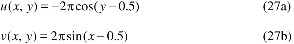
which represents a rigid body rotation with respect to(0.5,0.5) and the disk completes one revolution every unit time.

In the simulation, three different sets of grids (50×50, 100×100 and 200×200) are used to check the grid dependency of each method. After the first evolution cycle, the LS method causes a 9.48% loss of mass on a 50×50 grid and even with the finest resolution, the loss is still as high as 2.95%, and by increasing the grid resolution to 200×200, the error has dropped to 0.22%. The original CLS method shows much better mass conservation than the standard LS method. Furthermore, for the ICLS method, the error of the mass conservation is smaller than the CLS method at all grid resolutions with 1.28% of error on a 50×50 grid and 0.11% on a 200×200 grid (as shown in Table 1).

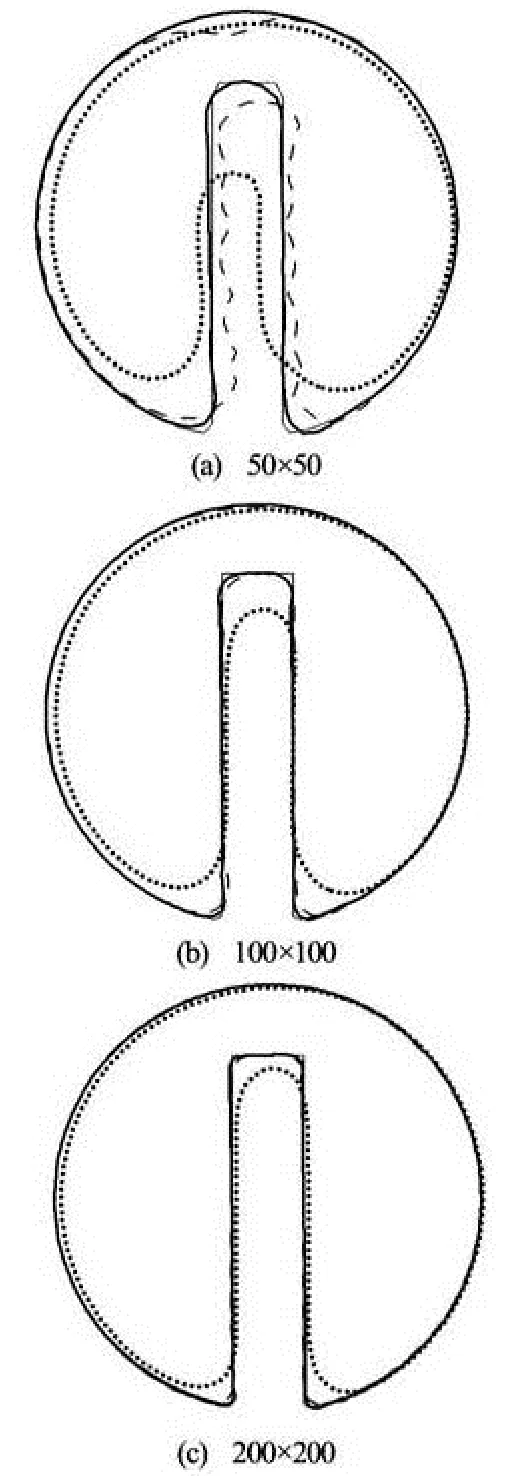
Fig.2 Zalesak’s disk problem, interface location obtained in the Zalesak’s disk test after one revolution with various grid sizes, using the different methods: The light solid line corresponds to the exact solution, the dark solid line to the ICLS method, the dashed line for CLS method, and the dotted line to the LS method

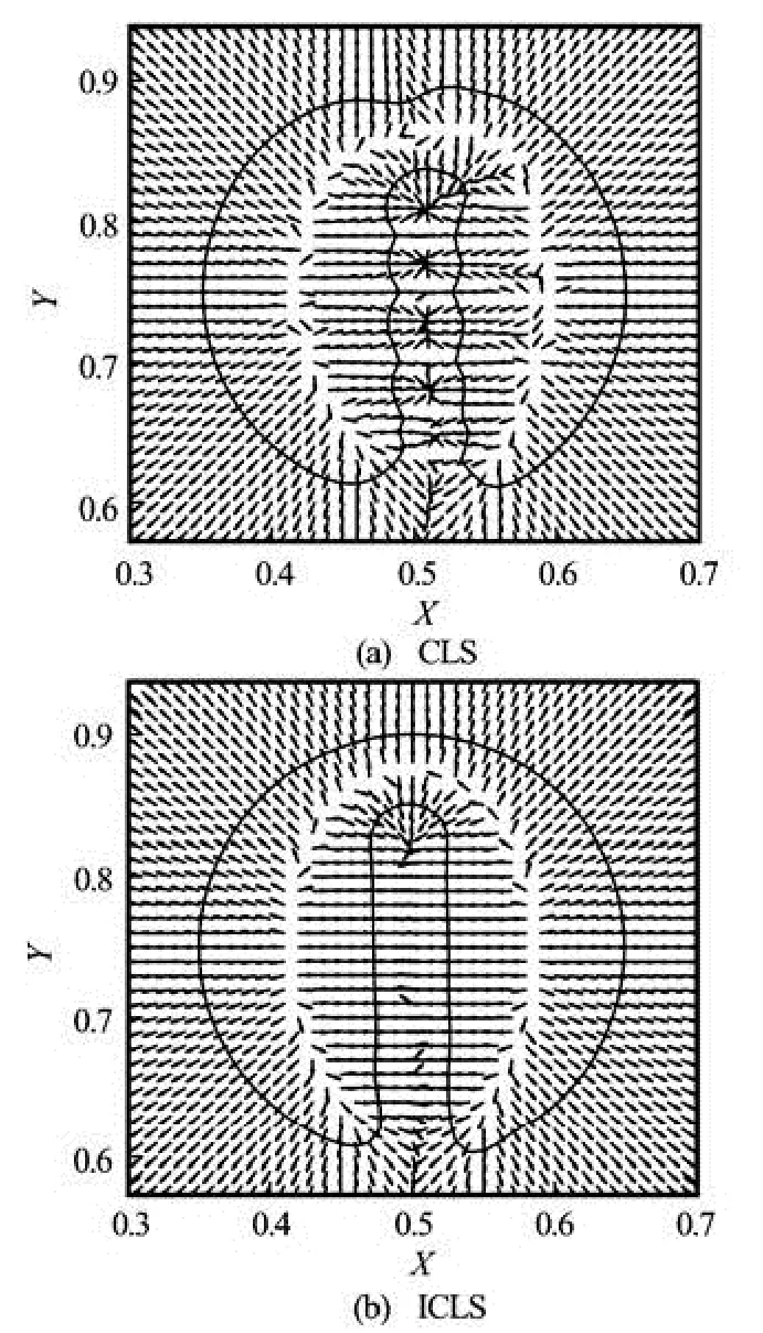
Fig.3 Zalesak’s disk problem, interface and normal direction after revolution with 50×50 grid

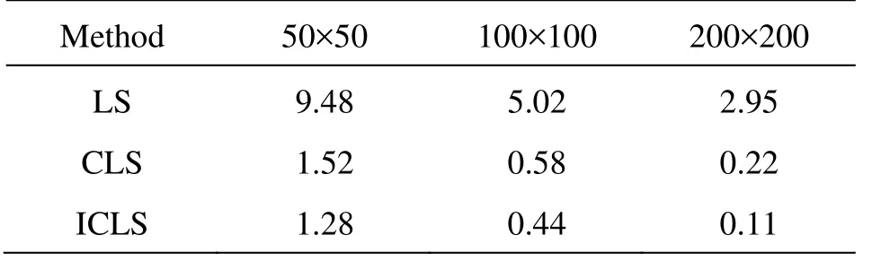
Table 1 Zalesak’s disk problem, percent relative mass errors after one revolution with various grid sizes (50× 50, 100×100 and 200×200), using the different methods:(LS, CLS and ICLS)

To further address this problem, the interface of the rotating disk after one cycle is plotted for the three methods. In Fig.2, the interface of the disk after one complete cycle is shown for different grid resolutions. It can be seen that with the 50×50 grid resolution, the interface from the level set and CLS methods has lost its original shape and becomes asymmetric with unsmoothness around the notch. The loss of symmetry of the interface is linked with the loss of the mass conservation in the corners which causes one side of the disk to evolve faster than the other. Also the unsmooth profile near the notch is due to the grid resolution and can be eased by increasing the grid resolution, as shown in Figs.2(b) and 2(c). On the 50×50 grid, there are only 3 grids between the notch sides and will lead to huge errors when calculating the surface normal for the CLS method. Figure 3 shows the surface normal for the CLS and ICLS cases on a 50×50 grid resolution. It can be seen that for the CLS case, the normal vectors near the notch point in various incorrect directions, which then cause “ripples” on the interface. However, for the same resolution, with thenormal vectors being calculated using the level set fun- ction φ, this problem is avoided.

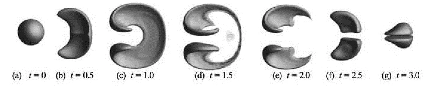
Fig.4 Sphere in deformation vortex, evolution of the interface at different time using CLS method under 1 003 uniform grids

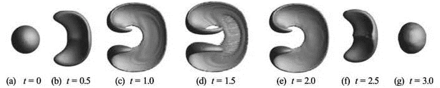
Fig.5 Sphere in deformation vortex, evolution of the interface at different time using ICLS method under 1 003 uniform grids

Based on the above discussion, the performance of the LS method is very poor in terms of the mass conservation and the shape preservation and is highly dependent on the grid resolution. The CLS method gives a good mass conservation and a shape preservation for the fine grid resolution but behaves badly when the grid becomes coarse. Thus, the accuracy of the CLS method also depends greatly on the mesh size and would require additional computational resources to handle complex flow problems. In overall, the ICLS method exhibits a better mass conservative feature and the interface profile matches perfectly with the exact solution for all grid resolutions.

3.2 Sphere in deformation vortex

The improvement of the present method over the original CLS method is further demonstrated by a 3-D sphere in the deformation vortex. The 3-D deformation field, is considered to be the most challenging conservation problem since it superposes similar deformation fields in the planes x-y and x- z, simultaneously imposing severe deformation states to the original shape[15]. This test case is used here to illustrate the robustness and conservative properties in a 3-D configuration. The interface is transported with the following velocity field,

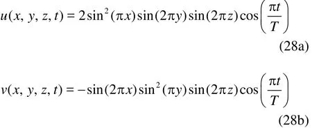
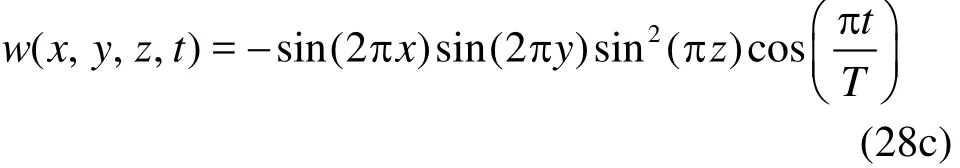
with a period T=3. The interface is initialized as a spherical drop of 0.15 in radius centered at the position (x=0.35, y=0.35 and z= 0.35) over a unit computational domain3[0,1]. The domain is discretized using 1003uniform grids. The sphere is stretched by two rotating vortices which initially scoop out the opposite sides of the sphere and then reverse them back to the initial shape. The deformed shapes reach the maximum stretching state at t=1.5 and after t= 1.5, the flow gradually returns back to the original state and the shapes is recovered to its initial shape at = t3.0.

The evolution of the sphere interface under 3-D deformation vortex using the CLS method and the ICLS method are shown in Figs.4 and 5, respectively. At the beginning, the opposite sides of the sphere are carved by two rotating vortices (= t0.5). And the vortices squeeze the sphere to a pancake form as shown in Figs.4 and 5 (t=1.0). Afterwards, the top and bottom sphere lobes are caught up with by the main vortices transforming the surface into a very slim and stretched shape (t=1.5). At this stage, the deformed shapes reach the maximum stretched state, and some part of the interface on both sides of the very stretched shape becomes as thin as the grid size, causing the collapse of the surface and the volume losses consequently. This phenomena is most significant in the case of the CLS method with a large void area as observed in Fig.6 at t=1.5 It is because that though the CLS method exhibits a good conservative property, it is difficult to resolve the thin interface. The shape of the stretched interface is shown in Fig.5 where the grid resolution is still not enough to resolve the thin membraneinterface. At t=1.5 only some ripples are observed at the thinnest area of the interface. And the result should be further improved by employing grids of a higher resolution.

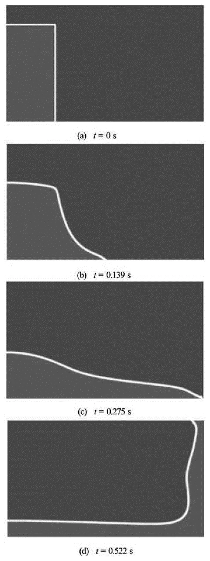
Fig.6 Dam break problem, snapshots of the water column in the middle of the tank at six typical times, t=0 s, 0.139 s, 0.275 s, and 0.522 s

After t=T/2, the flow field is reverted in order to recover the original shape of the sphere. At t=2.0, the shape of the interface from the ICLS method is recovered to a pancake profile while the interface from the CLS method falls into two parts implying a further loss of accuracy. At t=T, the sphere obtained by the ICLS method returns to its original shape with only a slight deformation. Under the same circumstances, the result from the CLS method has completely lost its initial shape and is split into two individual irregular shapes. Based on these observations, it can be concluded that the ICLS method is more suitable for problems with a complex geometry as it shows better capability to maintain the shape of the interface, as compared with the CLS method at the same grid resolution. Furthermore, the ICLS method also exhibits a better mass conservation property with the mass loss during a whole time period within 0.45% while with the CLS method, 6.5% of its original mass is lost.

3.3 Dam break flow

The dam-break problem is a popular validation case for various surface tracking and capturing methods because of the relatively simple geometry and initial conditions and the extensive experiment data and numerical results available. Martin and Moyce performed a benchmark laboratory experiment and many investigators have repeated the case either experimentally or numerically[13,16-20]. In this paper, a 3-D dam break problem is adopted to validate the proposed ICLS method by comparing the numerical results obtained against publishing experimental data and the case of ICLS methods, a great improvement on the numerical results.

The problem consists of a water column initially sustained by a dam, which is suddenly removed. The dimensions of the tank are 4a×a×2.4a and the dimensions of the water column are a×a×2a, where a=0.146 m. The density of water is 1 000 kg/m3and that of air is 1.2 kg/m3. The dynamic viscosity of water is set to 1.0×10-3kg/(ms) and that of air is 1.8× 10-5kg/(ms). The vertical acceleration due to gravity is taken to be 9.81 m/s2. Initially, the velocity is zero everywhere and the pressure is set to be the hydrostatic pressure. All boundaries of the tank are set as the free slip boundaries (zero normal velocity and zero tangential traction) except for the top boundary, which is assumed to be open (zero tangential velocity and zero normal traction). The mesh size adopted here is 160×40×96 (longitudinal×lateral×vertical).

It is noted that the free surface remains two-dimensional during the time interval of interest. Several snapshots of the water column in the middle of the tank are shown in Fig.6, and the key features of those snapshots from the simulation are:

t=0 s: initial state of the water column.

t=0.139 s: the front is propagated to the middle of the tank.

t=0.275 s: the front starts to hit the right wall of the tank.

t=0.522 s: the horizontal interface is almost parallel to the base of the tank and the water against the right wall has already fallen back under the influence of gravity, forming a vertical hump.

A more quantitative comparison for the early sta-ges of this experiment can be made by using the reduction in height and the speed of the wave front. The air-water interface position as a function of time on the bottom and the left walls of the tank is plotted in Fig.7. These results when compared to those given in literature[15,20]show that the proposed scheme is in good agreement with the experimental and numerical reference data. Good agreement with the experimental data is observed in the beginning of the water column collapse although at the later stages the computation results deviate from the experiment, which predicts a slower front propagation speed. Results presented by other researchers also show the same tendency and one reason for this is the difficulty in determining the exact position of the leading edge. Another reason for this discrepancy may be attributable to the fact that the free-slip boundary conditions are employed on the container surfaces, which is not possible to reproduce experimentally.

Fig.7 Dam break problem, position of air-water interface versus time in non-dimensional

4. Conclusion

An ICLS method is proposed for computing the free surface flows by coupling the standard LS method and the CLS method. The present ICLS method maintains the merit of good mass conservation of the CLS method while still being able to provide good approximations of the interface normal obtained by using the standard LS method. For all 2-D and 3-D benchmark cases considered, the results display both excellent mass conservation properties and good agreement with other existing experimental data and numerical results. The ability to capture the interface and maintain the sharpness of corners is demonstrated by Zalesak’s problem. The example of the sphere in the deformation vortex shows that the ICLS method could capture thin structures very well. After testing this technique against interface capture problems mentioned above, it is applied to a free surface flow simulation. The 3-D dam beak flow demonstrates the ability to deal with violent topological changes of the air/water interface.

[1] CIORTAN C., WANDERLEY J. B. V. and GUEDESSOARES C. Free surface flow around a ship model using an interface-capturing method[J].Ocean Engi-neering,2012, 44(4): 57-67.

[2] RAINALD L., CHI Y. and EUGENIO O. Simulation of flows with violent free surface motion and moving objects using unstructured grids[J].International Journal for Numerical Methods in Fluids,2007, 53(8): 1315- 1338.

[3] YU G., AVITAL E. J., and WILLIAMS J. J. R. Large eddy simulation of flow past free surface piercing circular cylinders[J].Journal of Fluids Engineering,2008, 130(10): 101304.

[4] TONY W. H. S., YU C. H. and CHIU P. H. Development of level set method with good area preservation to predict interface in two-phase flows[J].International Journal for Numerical Methods in Fluids,2011, 67(1): 109-134.

[5] Van DER PIJ S. P., SEGAL A., and VUIK C. et al. A mass-conserving level-set method for modelling of multi-phase flows[J].International Journal For Nu-merical Methods in Fluids,2005, 47(4): 339-361.

[6] DOUGLAS E., FRANK L. and RONALD F.. A fast and accurate semi-Lagrangian particle level set method[J].Computers and Structures,2005, 83(6): 479- 490.

[7] KOH C. G., GAO M. and LUO C. A new particle method for simulation of incompressible free surface flow problems[J].International Journal for NumericalMethods in Engineering,2012, 89(12): 1582-1604.

[8] SUSSMAN M. A second order coupled level set and volume-of-fluid method for computing growth and collapse of vapor bubbles[J].Journal of Computatio-nal Physics,2003, 187(1): 110-136.

[9] ELIN O., GUNILLA K. A conservative level set method for two phase flow[J].Journal of ComputationalPhysics,2005, 210(1): 225-246.

[10] ELIN O., GUNILLA K. and SARA Z. A conservative level set method for two phase flow II[J].Journal ofComputational Physics,2007, 225(1): 785-807.

[11] BARTO P. T., OBADIA B. and DRIKAKIS D. A conservative level-set based method for compressible solid/ fluid problems on fixed grids[J].Journal of Computa-tional Physics,2011, 230(21): 7867-7890.

[12] OWKES M., DESJARDINS O. A discontinuous Galerkin conservative level set scheme for interface capturing in multiphase flows[J].Journal of ComputationalPhysics,2013, 249(1): 275-302.

[13] KEES C. E., AKKERMAN I. and FARTHING M. W. et al. A conservative level set method suitable for variable-order approximations and unstructured meshes[J].Journal of Computational Physics,2011, 230(12):4536-4558.

[14] OLIVIER D., VINCENT M. and HEINZ P. An accurate conservative level set/ghost fluid method for simulating turbulent atomization[J].Journal of ComputationalPhysics,2008, 227(18): 8395-8416.

[15] RENATO N. E., and ALVARO L. G. A. C. Stabilized edge-based finite element simulation of free-surface flows[J].International Journal for Numerical Me-thods in Fluids,2007, 54(6-8): 965-993.

[16] CRUCHAGA M. A., CELENTANO D. J. and TEZDUYAR T. E. Moving-interface computations with the edge-tracked interface locator technique (ETILT)[J].International Journal for Numerical Methods in Fluids,2005, 47(6-7): 451-469.

[17] LOHNER R., YANG C. and ONATE E. On the simula-tion of flows with violent free-surface motion[J].Computer Methods in Applied Mechanics and Enginee-ring,2006, 195(41-43): 5597-5620.

[18] ELIAS R., COUTINHO A. Stabilized edge-based finite element simulation of free-surface flows[J].International Journal of Numerical Methods in Fluids,2007, 54(6-8): 965-993.

[19] LV X., ZOU Q. P. and ZHAO Y. et al. A novel coupled level set and volume of fluid method for sharp interface capturing on 3D tetrahedral grids[J].Journal of Com-putational Physics,2010, 229(7): 2573-2604.

[20] WEN X. Y. Wet/dry areas method for interfacial (free surface) flow[J].International Journal for Numerical Methods in Fluids,2013, 71(3): 316-338.

10.1016/S1001-6058(14)60035-4

* Project supported by the National Natural Science Foundation of China (Grant No. 51279050), the National High Technology Research and Development Program of China (863 Program, Grant No. 2012BAK10B04) and the Non-profit Industry Financial Program of Ministry of Water Resources of China (Grant No. 201301058)

Biography: ZHAO Lan-hao (1980-), Male, Ph. D., Professor

LIU Xiao-qing, Email: lxqhhu@163.com