
Comprehensive two-dimensional river ice model based on boundary-fitted coordinate transformation method
2014-03-06 06:21:57ZeyuMAOJingYUANJunBAOXiaofanPENGGuoqiangTANG
Water Science and Engineering 2014年1期
Ze-yu MAO*, Jing YUAN, Jun BAO, Xiao-fan PENG, Guo-qiang TANG
Department of Hydraulic Engineering, Tsinghua University, Beijing 100084, P. R. China
Comprehensive two-dimensional river ice model based on boundary-fitted coordinate transformation method
Ze-yu MAO*, Jing YUAN, Jun BAO, Xiao-fan PENG, Guo-qiang TANG
Department of Hydraulic Engineering, Tsinghua University, Beijing 100084, P. R. China
River ice is a natural phenomenon in cold regions, influenced by meteorology, geomorphology, and hydraulic conditions. River ice processes involve complex interactions between hydrodynamic, mechanical, and thermal processes, and they are also influenced by weather and hydrologic conditions. Because natural rivers are serpentine, with bends, narrows, and straight reaches, the commonly-used one-dimensional river ice models and two-dimensional models based on the rectangular Cartesian coordinates are incapable of simulating the physical phenomena accurately. In order to accurately simulate the complicated river geometry and overcome the difficulties of numerical simulation resulting from both complex boundaries and differences between length and width scales, a two-dimensional river ice numerical model based on a boundary-fitted coordinate transformation method was developed. The presented model considers the influence of the frazil ice accumulation under ice cover and the shape of the leading edge of ice cover during the freezing process. The model is capable of determining the velocity field, the distribution of water temperature, the concentration distribution of frazil ice, the transport of floating ice, the progression, stability, and thawing of ice cover, and the transport, accumulation, and erosion of ice under ice cover. A MacCormack scheme was used to solve the equations numerically. The model was validated with field observations from the Hequ Reach of the Yellow River. Comparison of simulation results with field data indicates that the model is capable of simulating the river ice process with high accuracy.
two-dimensional river ice numerical model; boundary-fitted coordinate technology; river ice process; freeze-up; MacCormack scheme; natural river
1 Introduction
The presence of ice in a river is an important phenomenon that should be considered in the development of water resources in cold regions. Ice formation can affect the design, operation, and maintenance of hydraulic engineering facilities. Major engineering concerns related to river ice are ice jam flooding, hydropower station operations, inland navigation, water transfers, and environmental, ecological, and morphological effects. The level of research activity on river ice has been disproportionally lower than that related to ice-free conditions. Although significant progress has been made in the last couple of decades, much more work still needs to be conducted.
Shen (1996) described the different river ice processes that may occur during a winter. River ice processes involve complex interactions between hydrodynamic, mechanical, and thermal processes. They are also influenced by weather and hydrologic conditions. Therefore, study of river ice evolution involves knowledge of river hydraulics, meteorology, thermodynamics, and geomorphology (Shen 2010).
Generally speaking, river ice mathematical models can be classified into two types: component models and comprehensive models (Shen 2010). Component models are mainly aimed at studying one or two specific river ice processes, used either to develop or to validate theoretical formulas and concepts, or to predict a specific river ice process. Information developed from component models can become the basis of comprehensive models.
On the other hand, comprehensive river ice models are capable of simulating the entire river ice regime. By utilizing existing theories, comprehensive river ice models capable of simulating all ice processes during a winter can be developed. Such a model can provide a continuous description of river ice evolution based on a limited amount of field data. It has been well recognized that such a numerical model can be the most economical tool for providing quantitative information for planning, design, and operations of river ice-related engineering projects. Most of the comprehensive models were initially developed for engineering needs related to the study of specific ice-related problems. With deepened understanding of the river ice physical phenomena and improvement in numerical methods, these early models show many limitations. As many ice processes are involved, it is crucial to have a coherent analytical framework when developing a comprehensive river ice model. Since almost all river ice phenomena are governed by thermal processes and ice transport, along with mechanical processes and phase changes, a coherent river ice model can be formulated with a thermal ice transport framework encompassing river ice evolution from freezing to breakup. Svensson et al. (1989) developed a model for thermal growth of border ice and presented a limiting condition for static border ice formation. Lal and Shen (1991) and Shen and Wang (1995) developed a two-layer analytical framework for river ice modeling based on the concept of thermal ice transport by treating the ice transport as a combination of the ice floating on the surface and the ice suspended over the depth of the flow beneath the surface ice. Anchor ice is included as a component and interacts with both the surface and suspended ice. Liu et al. (2006) established a two-dimensional comprehensive river ice model that includes all the major ice transport processes.
In the last thirty years or so, many researchers have developed theories related to ice evolution and presented a variety of comprehensive one-dimensional river ice models. Generally speaking, the one-dimensional river ice model is only applicable to straight channels and can only simulate the section-averaged values varying with time in the streamwise direction. For natural rivers, the water depth, velocity, and ice cover thickness vary dramatically in the transverse direction. It is therefore necessary to consider the characteristicvariations in the transverse direction in numerical simulation of river ice (Mao et al. 2008b).
The meandering banks of a natural river make it impossible to use rectangular Cartesian coordinates to deal with complex geometric boundaries accurately. The boundary-fitted coordinate (BFC) transformation method has been applied widely in many fields, such as environmental analysis, port and channel engineering, and flood control (Tan 1996). In order to accurately simulate complicated river geometry and overcome the difficulties of numerical simulation resulting from both complex boundaries and the difference between length and width scales, a comprehensive two-dimensional numerical model of river ice processes based on BFC, and including river hydraulics, ice transportation, thermodynamics, and freezing, was developed in this study.
2 Two-dimensional river ice mathematical model
The two-dimensional river ice mathematical model includes six major components: the river hydraulic model, water temperature model, surface ice and suspended frazil ice model, ice cover progression, ice transport under ice cover, and width of border ice.
2.1 River hydraulic model
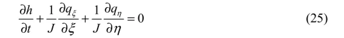
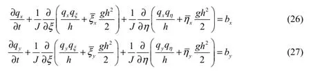
Two-dimensional shallow water equations in conservational form in terms of longitudinal coordinate x and transverse coordinate y were used as governing equations, with consideration of the resistance of the underside of the ice cover (Wang 1999):
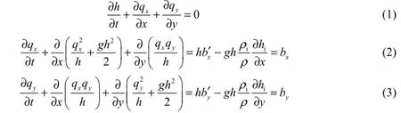
where ρ andiρ are the densities of water and ice, respectively; h is the water depth;ih is the ice cover thickness; g is the acceleration of gravity; t is time;xq andyq are the unit-width discharges in the x and y directions, respectively:xq hu= andyq hv= , with u and v being the flow velocity components in the x and y directions, respectively.
For an ice cover-free case:

For an ice-covered case:

where pais the atmospheric pressure at the water surface; zbis the elevation of the riverbed; τbis the riverbed resistance, and τb=τbxi +τbyj; τiis the resistance of theunderside of the ice cover, and τi=τixi +τiyj; τais the wind shear stress, and τa=τaxi +τayj =, where ρa(bǔ)is the air density, wais the wind speed, Cdis the non-dimensional coefficient of wind shear stress,and θais the angle between the wind velocity direction and the downstream direction of a river; Fbis Coriolis force, and Fb=Fbxi+ Fbyj, where Fbx= fv, and Fby=? fu; f is the coefficient of Coriolis force, and f = 2ω sinφ; φ is the latitude; and ω is the earth’s angular velocity: ω= 7.29× 10?5rad/s .
According to the Chezy formula, the riverbed resistance expression can bewhere R is the hydraulic radius, n is the Manning’s roughness coefficient, and w =u i +vj. For a wide and shallow river R ≈ h. Therefore, the riverbed resistance components in the x and y directions can be further simplified and expressed, respectively, as follows:

If ice cover is present, the total resistance of the underside of ice cover and the riverbed resistance in the x and y directions can be written, respectively, as

wherebn is the Manning’s roughness coefficient of the riverbed, andcn is the composite Manning’s roughness coefficient. There are a variety of expressions that can be used to calculatecn (Mao et al. 2002). In this study, the following Sababeev formula was used in calculation, for the sake of simplicity (Ashton 1986):
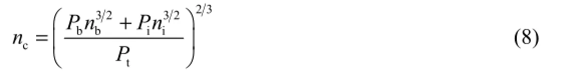
where niis the roughness coefficient of the underside of the ice cover; Pband Piare the wet perimeters of flow and ice cover, respectively; and Ptis the total wet perimeter: Pt= Pb+ Pi. For a wide and shallow river with ice cover, Pi≈ Biand Pb≈ Bo, where Biis the width of the ice cover, and Bois the width of the water surface.
2.2 Water temperature model
Water temperature of two-dimensional unsteady flows in terms of conservation of thermal energy can be written as (Yu 1988; Xu 2007)
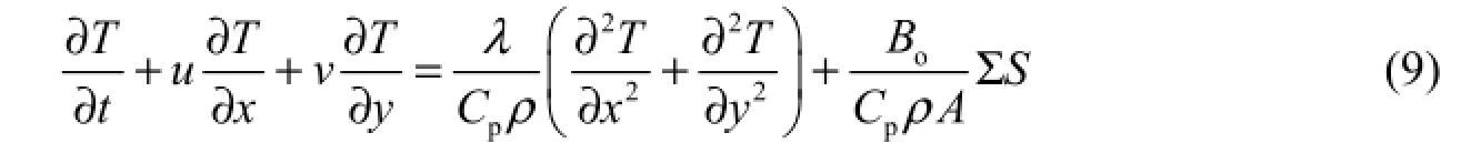
where T is the depth-averaged water temperature,pC is the specific heat of water, A is the cross-sectional area of flow, λ is the thermal conductivity of water, and SΣ is the net heat flux per unit flow surface area.
For the convenience of deducing the governing equations on a curvilinear grid, the aboveequation can be rewritten as follows:

wherexJ andyJ are thermal flux components in the x and y directions, respectively:; and Γ is the heat dispersion coefficient:
2.3 Surface ice and suspended frazil ice model
According to the two-layer ice transport theory, the river ice can be divided into the surface ice and suspended frazil ice in the ice cover-free river reach. The equations for surface and suspended frazil ice concentrations are, respectively (Wang 1999):
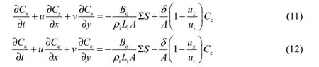
where Csis the concentration of surface ice; Ccis the concentration of suspended frazil ice; Liis the latent heat of fusion; δ is the an empirical coefficient quantifying the rate of supply to surface ice from suspended frazil ice (Wu 2002); uiis the buoyant velocity of ice particles, and, wheresT is the water temperature at the water surface; andzu is the vertical velocity component due to flow turbulence, andwhere C is the Chezy coefficient.
2.4 Ice cover progression
Depending on the hydraulic condition at the leading edge of the ice cover, there are three kinds of ice cover progression modes: the juxtaposition mode, hydraulic thickening (narrow jam) mode, and mechanical thickening (wide jam) mode. According to the mass conservation of surface ice at the leading edge, the rate of ice cover progression in terms of unit-width discharges is (Xu 2007)
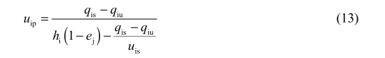
where ejis the overall porosity of ice cover, and ej= ep+ (1 ? ep)ec, where epis the porosity between ice floes and ecis the porosity of an ice floe; qiuis the unit-width discharge of ice entrained under the ice cover at the leading edge (m2/s); qisis the unit-width ice discharge in the surface ice layer (m2/s), and qis= Csq, where q is the unit-width water discharge; and uisis the velocity of the incoming surface ice. The node-isolation method isapplied in computation, i.e., by regarding the grid point as a control unit, the progression distance of each grid point at the leading edge is calculated (Mao et al. 2003, 2004).
When the Froude number at the leading edge Fr is less than a critical Froude number Frc, the ice cover will progress upstream in the juxtaposition mode. The critical Froude number Frccan be expressed as
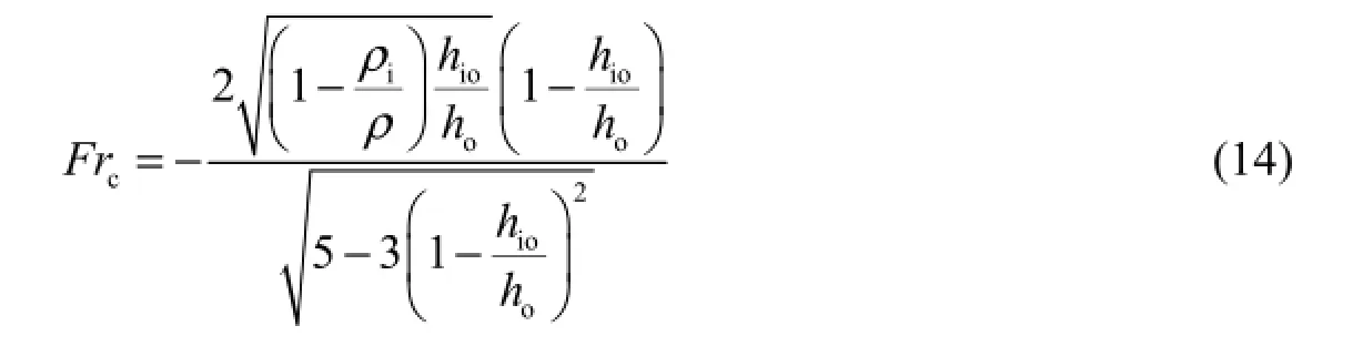
where hois the water depth at the leading edge of ice cover, and hiois the thickness of the incoming floe. The Froude number at the leading edge Fr is defined as
By contrast, if Fr is greater than Frc, single floe juxtaposition cannot be maintained. At this time, the upstream incoming ice will be entrained under the ice cover, resulting in a narrow jam, and the ice cover will progress upstream in the hydraulic thickening (narrow jam) mode, inducing the thickness of ice cover to increase, the water level at the leading edge to rise, and flow at the bottom to separate.
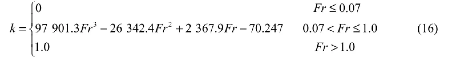
The dive coefficient (k) of incoming ice at the leading edge can be defined in terms of unit-width discharges as (Wang 1999)
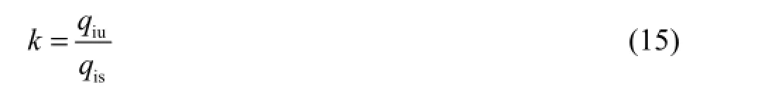
It is difficult to determine the k value according to Eq. (15), and we adopt the following formula:
According to ice conservation, the change of the thickness of ice cover in a river with a length of xΔ during a period of tΔ is

As the thickness of ice cover at the leading edge increases, the Froude number gradually decreases. When the Froude number is less thancFr, the leading edge of ice cover will progress again.
If forces acting on the ice cover exceed the bank shear stress, mechanical thickening will occur, and the balance thickness of the ice coveribh can be calculated with Eq. (18) (Xu 2007):

whereuu is the velocity under the ice cover, μ is the friction coefficient between floes ( 1.28μ= ),DR is the hydraulic radius of ice-covered flows,cτ is the cohesion term of thebank shear stress, anduh is the water depth underneath ice cover.
2.5 Ice transport under ice cover
The ice transport capacity is formulated in the following relationship (Shen and Wang 1995):

where ? is the dimensionless ice transport capacity, andwhere qiis the ice volumetric discharge per unit width, dnis the nominal diameter of ice particles, F is the fall velocity coefficient, and Δ= 1? ρiρ; Θ is the dimensionless flow strength, andwhere V is the shear velocity on the underside of the ice cover; Θ is*icthe dimensionless critical shear stress.
2.6 Width of border ice
Border ice will initially form, if the depth-averaged velocity component near the border in the x direction (su) satisfies the following condition (Ashton 1986):
The border ice will also progress in the transverse direction due to the congregation of incoming floes. Depending on stabilization between floes and border ice, the progression rate of border ice is calculated as follows:

where WΔ is the increased width of border ice during a given period, andcu is the maximum allowable velocity at which a floe can adhere to the existing border ice.
3 Transformation of boundary-fitted coordinate system
3.1 Grid generation
The coordinates of a point in the physical plane are denoted by (x, y), and the coordinates of a point in the computational plane are denoted by (ξ, η). In order to make the computational grid accurately fit the boundaries of the computational domain, the irregular domain enclosed by complex boundaries on the physical plane (x-y plane) is transformed into a rectangular domain on the computational plane ( ξ-η plane) through coordinate transformation, as shown in Fig. 1, where D*is the computational domain in ξ-η coordinates; D is the computational domain in x-y coordinates; and Γ1*(ξ = 1), Γ2*(η = 1), Γ3*(ξ = N), and Γ4*(η = M) are the boundaries of D*, corresponding to the boundaries Γ1, Γ2, Γ3, and Γ4of D, respectively. By solving the elliptic partial differential equations, the coordinates on the ξ-η plane corresponding to those on the x-y plane can be obtained: ξ= ξ(x ,y )and η= η (x ,y), which satisfy the following equation (Xu 2007; Mao et al. 2008a; Liang 1998):and the Dirichlet boundary conditions, where P and Q are both continuous functions of ξ and η. By selecting proper values of P and Q, curvilinear grids with various densities on the x-y plane can be transformed into uniform rectangular grids on the -ξη plane.

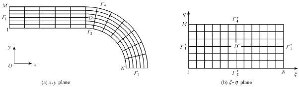
Fig. 1 Computational domains in x-y plane and -ξη plane
The procedure of BFC generation includes arrangement of grid points along boundaries of the domain D on the x-y plane. As shown in Fig. 1(a), M nodes are arranged along boundaries Γ1and Γ3, N nodes are arranged along boundaries Γ2and Γ4, and the spacing between those nodes can be unequal. Nodes at boundaries of the domain D*correspond to nodes at boundaries of the D domain. Then, with the chain-derivative method, the following equations are numerically solved using the central difference scheme:

3.2 Transformation of governing equations
Similarly, by transformation of Eqs. (10) through (12), the aforementioned governing equations of water temperature, and concentrations of surface and frazil ice under the BFC system can be deduced:

3.3 Transformation of boundary conditions
The boundary conditions can be generally expressed asa1φ+ b1(?φ ? n )=c1, where a1, b1, and c1are given values, n is the outward unit normal vector of the boundary, φ is an unknown variable, and the gradient of an arbitrary function f is ?f= ( fξξx+ fηηx)i + ( fξξy+fηηy)j. If f = ξ, and f =η , the transformed forms of boundary conditions can be obtained as follows:

whereξn andηn are the unit vectors pointing in the positive ξ and ηdirections, respectively.
4 Numerical methods
As illustrated in Fig. 2, the control volume is denoted by ABCD, (i, j) is a control node, and the control area is denoted by ξηΔΔ .
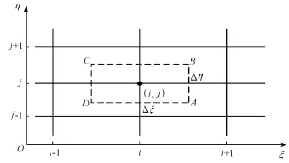
Fig. 2 Sketch of control volume
Eqs. (25) through (30) can be expressed in the following vector forms:
Its general discretization form is as follows:

where HAB= FABΔη, HBC= GBCΔξ, HCD=? FCDΔη, and HDA=?GDAΔξ, with FAB= (Fi+1,j+ Fi,j)2,GBC=(Gi,j+1+Gi,j)2,FCD=(Fi?1,j+Fi,j)2, and GDA=(Gi,j?1+Gi,j)2.
A two-step MacCormack scheme was used to solve the above equations. In order to assure symmetry of computation, stagger arrangement of forward and backward difference was adopted at control surfaces in the ξ and η directions. Node variables were staggered, which was helpful to solving the moving boundary conditions.
5 Model test
5.1 Hequ Reach of Yellow River
Field observations (HFPDFHC 1993) in the Hequ Reach of the Yellow River were used to validate the numerical model. A sketch of the Hequ Reach is shown in Fig. 3. It was concluded from the original observations that the ice cover formation and evolution in the Hequ Reach of the Yellow River involve two processes. First, the ice cover continuously progresses upstream and freezes up. Second, the leading edge of the ice jam stops developing upstream after the ice jam advances to near Longkou, and then turns into the late evolution stage, because of rapid flow in the canyon upstream. Because of a lack ofcross-section data upstream of Longkou, these two processes were simulated separately. The numerical simulation of the freeze-up process was conducted in the reach from Longkou to Yumiao, with a length of 58.5 km (19 cross-sections in total), and the computations were compared with field observations. Characteristics of cross-sections of the Hequ Reach are shown in Table 1.
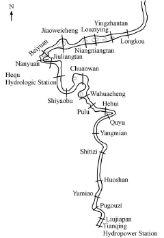
Fig. 3 Sketch of Hequ Reach of Yellow River
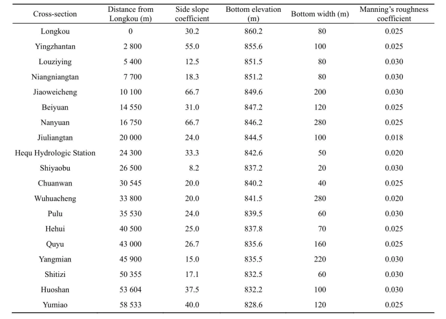
Table 1 Characteristics of cross-sections of Hequ Reach
For the freeze-up process, the period of time simulated was three days, from 8:00 am on November 26 to 8:00 am on November 29, 1986. The time step was 900 seconds. The upstream and downstream boundary conditions were the flow rate hydrograph and water level hydrograph, respectively. For the late evolution process, the period of time simulated was 80 days, from 8:00 am on December 11, 1986 to 8:00 am on March 1, 1987. The time step was 3 600 seconds. Boundary conditions were the upstream flow rate hydrograph, thickness of the ice jam of the upstream section, and downstream water level hydrograph.
5.2 Grid division
There are bends, islands, and shoals in the Hequ Reach. The shoals divide the river reach into several sub-rivers, and the boundary of the adjacent sub-rivers is composed of the boundary of shoals and the public water boundary. The whole computational area was made up of multiple connected zones. For every sub-river, a structured grid was established usingthe structured joining method (Xu 2007). During the computation process, calculation on the locally refined grid and initial grid was conducted separately with the same method. First, the area of the original grid that needed to be locally refined was selected. Then, every grid in the selected area was divided into DI× DJlocally refined grid cells, where DIis the grid-refined coefficient in the x direction, and DJis the grid-refined coefficient in the y direction. In this study, DI= DJ= 4. The computational area was divided into three reaches: the open-flow reach, progression reach, and ice-cover reach. The grid was re-divided depending on the progressive distance of the leading edge. In this study, x represents the streamwise direction, y represents the transverse direction, and the origin is on the right bank of the Longkou cross-section. The initial BFC grid was divided into 1 000 × 20 cells. After the grid was refined, the maximum grid cell size was 80.5 m, and the minimum grid cell size was 2.6 m. Fig. 4 shows the computational grid. Fig. 5 shows the calculation procedure, whereNs=max (DI,DJ), Niis the number of space steps of ice-cover reach, and N0is the number of space steps of open-flow reach.
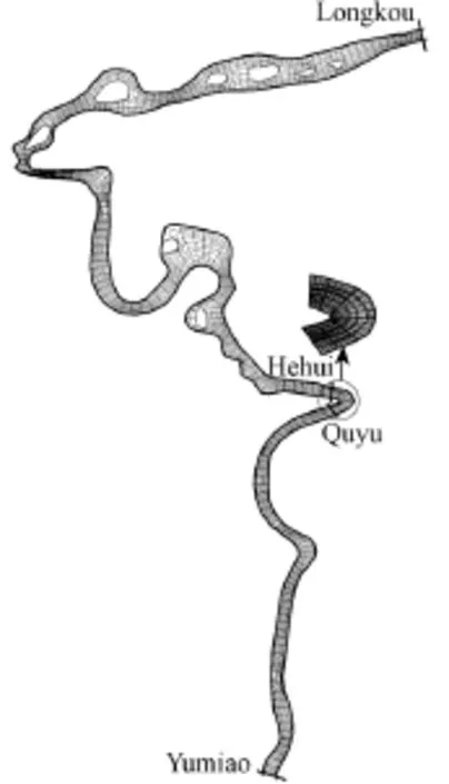
Fig. 4 Computational grid
5.3 Simulation results and analysis
Fig. 6 shows the calculated water levels and field observations during the freeze-up period. It is obvious that the water level at the leading edge of the ice cover increased as the ice cover advanced. Water level variations in the transverse direction are shown in Fig. 7, which indicates that the numerical simulations are in agreement with observations.
Fig. 8 provides a comparison between computations and field observations of the position of the leading edge of the ice cover. It can be found that the computations are in agreement with field observations, and the progression speed of ice cover in the transverse direction is not uniform. The main reason may be that the floe concentration at the leading edge of the ice cover is largely affected by air temperature.
Fig. 9 compares computations and field observations of thickness of ice cover. It can be seen that, during the ice cover progression, the thicknesses of ice cover in different reaches are not consistent. The main reason is that the geometric characteristics of each cross-section, incoming ice, and flow conditions are not the same when the ice cover initially forms, and the ice transportation under ice cover causes the thickness of downstream ice cover to change. Besides, the results of research show that the mechanical thickening mode occurs during the ice cover progression, and the reason is that the width of the cross-section is much larger than the water depth in the bending reach.

Fig. 5 Flowchart of calculation procedure

Fig. 6 Comparison of measured and computed water levels (z) at different times and comparison of them and initial values
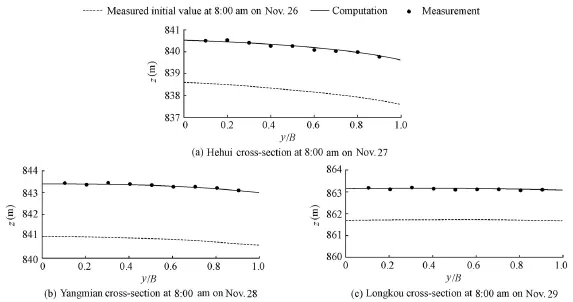
Fig. 7 Comparison of measured and computed water levels (z) at different cross-sections and times and comparison of them and initial values
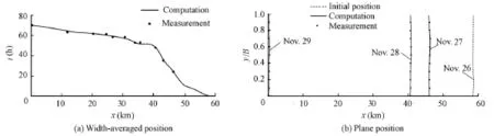
Fig. 8 Variation of position of leading edge of ice cover
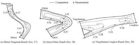
Fig. 9 Ice cover thickness in different reaches
6 Conclusions
In order to accurately simulate the complicated boundary conditions in natural rivers, a two-dimensional numerical model of river ice processes was developed, based on boundary-fitted coordinates. The MacCormack scheme was used to solve the transformed equations. The model was validated with field observations from the Hequ Reach of the Yellow River, and satisfactory results were achieved. This study shows that the progression rate of the ice-cover leading edge and the thickness distribution of ice cover are affected by many factors, and the water level at the leading edge of the ice cover increases while the leading edge advances upstream.
Ashton, G. D. 1986. River and Lake Ice Engineering. Littleton: Water Resources Publications.
Headquarters of Flood Prevention and Draught Fighting of Hequ Country (HFPDFHC). 1993. Collection of Observational Data on the Hequ Reach of Yellow River, Shanxi Province. Hequ: Yellow River Water Conservancy Press. (in Chinese)
Lal, A. M. W., and Shen, H. T. 1991. Mathematical model for river ice processes. Journal of Hydraulic Engineering, 117(7), 851-867.
Liang, K. M. 1998. Mathematical Physical Method. 3rd ed. Beijing: Higher Education Press. (in Chinese)
Liu, L. W., Li, H., and Shen, H. T. 2006. A two-dimensional comprehensive river ice model. Proceedings of the 18th IAHR International Symposium on Ice, 69-76. Sapporo: Hokkaido University Press.
Mao, Z. Y., Ma, J. M., She, Y. T., and Wu, J. J. 2002. Hydraulic resistance of ice-covered river. Journal of Hydraulic Engineering, 33(5), 59-64. (in Chinese) [doi:0559-9350(2002)05-0059-06]
Mao, Z. Y., Zhang, L., Wang, Y. T., and Wu, J. J. 2003. Numerical simulation of river-ice processes using boundary-fitted coordinate. Journal of Glaciology and Geocryology, 25(s2), 214-219. (in Chinese)
Mao, Z. Y., Zhang, L., and Yue, G. X. 2004. Two-dimensional model of river-ice processes using boundary-fitted coordinate. Proceedings of the 17th IAHR International Symposium on Ice, Vol 1, 184-190. St. Petersburg: B. E. Vedeneev All-Russia Research Institute of Hydraulic Engineering (VNIIG).
Mao, Z. Y., Xu, X., Wang, A. M., Zhao, X. F., and Xiao, H. 2008a. 2D numerical model for river-ice processes based upon boundary-fitted coordinate. Advances in Water Science, 19(2), 214-223. (in Chinese)
Mao, Z. Y., Zhao, X. F., Wang, A. M., Xu, X., and Wu, J. J. 2008b. Two-dimensional numerical model for river-ice processes based upon boundary-fitted coordinate transformation method. Proceedings of the 19th IAHR International Symposium on Ice, Using New Technology to Understand Water-Ice Interaction,191-202. Vancouver: IAHR.
Shen, H. T., and Wang, D. S. 1995. Under cover transport and accumulation of frazil granules. Journal of Hydraulic Engineering, 121(2), 184-195.
Shen, H. T. 1996. River ice processes: State of research. Proceedings of the 13th International Symposium on Ice, Vol 3, 825-833. Beijing.
Shen, H. T. 2010. Mathematical modeling of river ice processes. Cold Regions Science and Technology, 62(1), 3-13. [doi:10.1016/j.coldregions.2010.02.007]
Svensson, U., Billfalk, L., and Hammar, L. 1989. A mathematical model of border ice formation in rivers. Cold Regions Science and Technology, 16(2), 179-189. [doi:10.1016/0165-232X(89)90019-0]
Tan, W. Y. 1996. Computational Methods for Shallow-water Dynamics: Applications of FVM. Beijing: Tsinghua University Press. (in Chinese)
Wang, Y. T. 1999. Numerical Simulation of River Ice and Analysis of Ice Characteristics During Water-transfer in Winter. Ph. D. Dissertation. Beijing: Tsinghua University. (in Chinese)
Wu, J. J. 2002. Ice Processes Mechanism and Numerical Simulation of Ice Jam and Frazil Ice Evolution. M. E. Dissertation. Beijing: Tsinghua University. (in Chinese)
Xu, X. 2007. Study of 2D BFC Numerical Model of River-ice Processes and Velocity Distributions of Ice-covered Flow. M. E. Dissertation. Beijing: Tsinghua University. (in Chinese)
Yu, Z. P. 1988, Theory of Heat Transfer. 2nd ed. Beijing: Higher Education Press. (in Chinese)
(Edited by Yan LEI)
——
This work was supported by the National Natural Science Foundation of China (Grant No. 50579030).
*Corresponding author (e-mail: maozeyu@tsinghua.edu.cn)
Received Jul. 25, 2012; accepted Nov. 14, 2012
 Water Science and Engineering2014年1期
- Water Science and Engineering的其它文章
- Thank you to our peer reviewers
- Water issues and prospects for hydrological science in China
- Abrasion test of flexible protective materials on hydraulic structures
- Performance of a double-layer BAF using zeolite and ceramic as media under ammonium shock load condition
- Prediction of chlorophyll a concentration using HJ-1 satellite imagery for Xiangxi Bay in Three Gorges Reservoir
- Water level updating model for flow calculation of river networks